Optimizing 70B Model Serving on 4xH100: Memory & Communication Trade-offs

Introduction

Welcome back. In our previous lesson, we analyzed the distinct communication patterns of tensor and pipeline parallelism, concluding with a crucial rule of thumb: use tensor parallelism (TP) within a node to leverage fast interconnects like NVLink, and use pipeline parallelism (PP) to scale across nodes.

This lesson is the culmination of our work on distributed inference. Your goal is to apply this knowledge to a concrete system design problem: Determine an optimal parallelism configuration for serving a 70B model on a 4xH100 cluster based on memory and communication trade-offs.

You will step into the role of an AI Systems Engineer and make a data-driven decision. We will walk through a multi-stage analysis, starting with basic memory feasibility and refining our choice based on performance metrics and workload characteristics. This process will solidify your mental model for how to configure distributed systems in production.

1. The Design Problem: Scoping and Specifications

First, let's define the components of our system design problem.

• Model: A generic 70-billion parameter decoder-only transformer. We'll assume it's being served at bfloat16 precision.
• Hardware: A "4xH100 cluster". In industry terms, this typically refers to a single server (a single node) containing four H100 GPUs.
• Interconnect: We can assume these H100s are within a single node and connected via high-speed NVLink.

Our task is to choose the values for tensor_parallel_size and pipeline_parallel_size.

Before diving into the analysis, let's review the hardware specs and key parallelism concepts from a practical perspective.

2. Stage 1: Memory Feasibility Analysis

The first and most important constraint is memory. An LLM deployment has three main memory consumers: model weights, KV cache, and framework overhead. If the model weights alone don't fit, no amount of performance tuning matters.

1. Calculate Model Weight Size:

   • Parameters: 70 billion
   • Precision: bfloat16 (2 bytes per parameter)
   • Total Weight Size: $70\times 10^9\text{ params}\times 2\text{ bytes/param}=140\times 10^9\text{ bytes}\approx 140\text{ GB}$
     (Note: 1 GB = $10^9$ bytes, while 1 GiB = $2^{30}$ bytes. We'll use GB for simplicity here, which is common for back-of-the-envelope calculations.)

2. Evaluate Possible TP Configurations:

   • GPU VRAM: An H100 has 80 GB.
   • Minimum GPUs: $\frac{140\text{ GB (weights)}}{80\text{ GB/GPU}}\approx 1.75$. This immediately tells us that we need at least 2 GPUs. TP=1 is impossible.

Let's analyze the memory pressure for the viable options on our 4-GPU system:

Configuration	# GPUs	Total GPUs	Weights per GPU	Remaining VRAM per GPU	Feasibility
TP=2, PP=1	2	2 of 4	$140\text{ GB}/2=70\text{ GB}$	$80-70=10\text{ GB}$	Risky. Leaves very little room for KV cache, activations, and framework overhead.
TP=3, PP=1	3	3 of 4	$140\text{ GB}/3\approx 46.7\text{ GB}$	$80-46.7\approx 33.3\text{ GB}$	Technically possible, but TP sizes are often powers of 2 for efficiency.
TP=4, PP=1	4	4 of 4	$140\text{ GB}/4=35\text{ GB}$	$80-35=45\text{ GB}$	Viable. A comfortable amount of VRAM remains for dynamic allocations.
TP=2, PP=2	2 per stage	4 of 4	See below	See below	A hybrid option to consider.

For the TP=2, PP=2 case, the model's layers are split in half. Each pipeline stage handles ~35B parameters, or 70 GB of weights. Each stage then uses TP=2, so each GPU holds $70/2=35\text{ GB}$ of weights. The memory footprint per GPU is identical to the TP=4, PP=1 case.

Conclusion from Stage 1: From a memory perspective, TP=4 is the most robust configuration, providing ample headroom. TP=2 is too tight and risks Out-Of-Memory (OOM) errors once KV cache for even a moderate batch size is allocated.

3. Stage 2: Performance Trade-off Analysis

Now that we've narrowed our choices to TP=4, PP=1 and TP=2, PP=2, let's analyze their performance characteristics based on what we learned in the last lesson. We are on a single node with fast NVLink.

• Configuration 1: TP=4, PP=1

  • Compute: Excellent. All 4 GPUs work in parallel on each layer. There is no pipeline bubble.
  • Communication: Requires an all-reduce collective operation across all 4 GPUs for each parallel block in the model. This incurs communication overhead, but it happens over very fast NVLink.

• Configuration 2: TP=2, PP=2

  • Compute: Sub-optimal. This configuration introduces a pipeline bubble, meaning GPUs in one stage will be idle while waiting for the other. Even with micro-batching, this fundamentally reduces total compute utilization.
  • Communication:
    • Within each stage, all-reduce only occurs across 2 GPUs, which is faster than a 4-GPU all-reduce.
    • Between stages, a send/recv point-to-point operation is required. Over NVLink, this is extremely fast.

The Decisive Factor:
The core trade-off here is TP=4's communication overhead vs. TP=2, PP=2's compute bubble.

Given that all communication is happening over a high-performance, low-latency NVLink fabric, the penalty for a 4-way all-reduce is significant, but manageable. In contrast, the pipeline bubble represents a guaranteed loss of computational power. For a shallow pipeline of only two stages, this bubble can be quite substantial.

Therefore, to maximize GPU utilization on a single, well-connected node, avoiding the pipeline bubble is the top priority.

Conclusion from Stage 2: The TP=4, PP=1 configuration is superior because it avoids introducing a pipeline bubble, which would be a greater source of inefficiency than the communication overhead of a 4-way all-reduce over NVLink.

4. Stage 3: Workload-Specific Tuning & Validation

We've established TP=4 as our optimal configuration. Now, let's validate this decision and consider how different workloads might affect it. An AI Systems Engineer always looks for data to support their design choices.

Latency vs. Throughput

The article "LLM Inference Performance Engineering: Best Practices" provides empirical data for a 70B model.

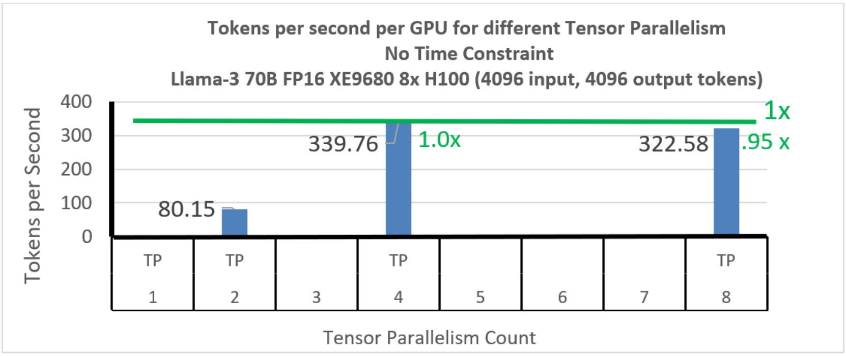
The data shows that while more TP reduces latency, the gains diminish. This is because at some point, the communication overhead of all-reduce begins to cancel out the computational speedup. This reinforces that TP=4 is a strong choice, likely hitting a sweet spot on the performance-per-GPU curve.

The Role of KV Cache

What if our workload requires extremely long context lengths or very high concurrency? This would demand a massive KV cache. The Anyscale documentation provides a perfect worked example.

This example validates our TP=4 decision for general-purpose and low-latency use cases. It also introduces an important tuning concept: if your primary bottleneck becomes KV cache capacity, you can increase tensor_parallel_size further (if you have more GPUs) to shrink the per-GPU weight footprint, thereby freeing up more memory for the cache. On our 4xH100 system, TP=4 is the maximum possible, so it's the best we can do for both latency and throughput.

Final Recommendation

After a three-stage analysis, we can confidently determine the optimal configuration.

Final Answer: For serving a 70B model on a single 4xH100 node, the optimal configuration is tensor_parallel_size=4 and pipeline_parallel_size=1.

Justification Summary:

1. Memory: TP=4 allocates 35 GB for weights per GPU, leaving a healthy 45 GB for KV cache and overhead, comfortably fitting the model and supporting high-throughput workloads. TP<4 would create significant memory pressure.
2. Performance: TP=4, PP=1 avoids the compute inefficiency of a pipeline bubble. On a single node with fast NVLink, this is more important than the added communication overhead of a 4-way all-reduce compared to a hybrid TP=2, PP=2 setup.
3. Validation: Empirical data confirms that TP=4 is a "sweet spot" for 70B models, providing excellent latency with diminishing returns for higher TP degrees. It also maximizes the available VRAM for KV cache on a 4-GPU system, making it suitable for high-throughput scenarios.

Conclusion

In this lesson, you synthesized everything you've learned about distributed inference to solve a realistic system design problem. You saw how to reason from first principles, starting with hard constraints like memory and progressively refining your decision based on performance trade-offs and workload characteristics.

Key Takeaways:

• System design is a process of elimination and refinement: Start with what's possible (memory), then optimize for what's efficient (performance trade-offs), and finally tune for the specific use case (workload).
• Memory is the first gate: Always perform a back-of-the-envelope calculation of weight size vs. VRAM to determine the minimum required degree of parallelism. A 2x safety factor over minimum weights is a good rule of thumb.
• Avoid bubbles on fast interconnects: Within a single, NVLink-connected node, prioritize maximizing compute utilization by avoiding pipeline parallelism if possible.
• Use data to validate your design: Your reasoning should be supported by empirical benchmarks and best-practice guides from industry leaders whenever possible.

Preview of the Next Lesson:

You have now designed a distributed serving setup on paper. The next step is to see how these concepts are implemented in the real world. In the next module, "Evaluating Production Inference Frameworks," we will begin by deploying a model using vLLM, one of the most popular open-source inference servers. You will benchmark its throughput, latency, and GPU utilization, connecting the theoretical designs we've discussed to concrete, measurable performance.