Acceptance Criteria for Successful Runs and Trustworthy Differential-Expression Results

Hello. In the previous lesson, you made your pipeline’s hidden contracts visible: assumptions in filenames, directories, metadata, and reference resources. This lesson turns those contracts into acceptance criteria: explicit, testable conditions that tell you whether a run is complete enough to use and whether a differential-expression result is defensible enough to report.

For a job-ready RNA-seq portfolio, “the script finished” is not a sufficient success criterion. A credible project can show what was checked, which thresholds were used, why they fit the dataset, what happened when a threshold was missed, and which outputs remain valid. By the end of this lesson, you should be able to write a compact acceptance-criteria document for your own analysis.

---

Acceptance criteria are decision rules, not a collection of plots

An acceptance criterion has five parts:

1. Metric: what you measure.
2. Rule or threshold: what counts as pass, warning, or hold.
3. Scope: which samples, genes, or runs the rule applies to.
4. Action: what you do when the rule is not met.
5. Evidence: the file, plot, log, or table that records the decision.

For example, this is not yet an acceptance criterion:

“Check mapping rate.”

This is measurable:

“For a human bulk RNA-seq library aligned to the documented reference, unique mapping rate of at least $75\%$ is a pass; $60\%$ to less than $75\%$ requires review; below $60\%$ puts the analysis on hold until the cause is investigated. Record the rate in the MultiQC summary.”

The threshold is not universal. It depends on the organism, assay, reference quality, and aligner or quantifier. But the decision policy should be explicit before you interpret results.

It is useful to separate two gates:

Gate	Question answered	Typical evidence
Successful pipeline run	Did the workflow process the intended inputs completely and produce technically credible outputs?	Logs, checksums, FastQC, MultiQC, mapping summaries, count matrix
Trustworthy DE result	Does the count matrix, metadata, model, and result table support the stated biological comparison?	Metadata validation, sample-distance plot, PCA, DESeq2 diagnostics, documented contrast, annotated results table

A run can pass the first gate yet fail the second. For example, an aligner may successfully produce BAM files for every sample, while the metadata reveal that all controls were sequenced in one batch and all treatments in another. Conversely, a biologically sensible design cannot rescue an incomplete run with missing samples or mismatched count columns.

Pass, warning, and hold

Use three statuses rather than treating every non-ideal metric as a failure:

• Pass: meets the stated criterion; proceed.
• Warning / review: does not meet an expected pattern, but may be explainable; inspect and document a decision.
• Hold: a condition that can invalidate the analysis or its interpretation; do not proceed until resolved or explicitly redefine the analysis scope.

This distinction matters for bulk RNA-seq. A high duplication rate, unusual GC distribution, or a FastQC warning can be biologically plausible. The professional response is not automatic deletion; it is targeted investigation.

---

Technical acceptance: did the run produce credible inputs for counting?

Before deciding whether genes are differentially expressed, establish that the computational run itself is complete, traceable, and technically plausible.

Start with completeness and identity

The first checks are deliberately unglamorous, but they prevent many silent errors.

Criterion	Pass condition	Hold condition	Evidence to retain
Input identity	Every expected analysis_sample_id has the required FASTQ input or documented public-data equivalent.	Missing input, unexpected extra sample, broken read pair, or ambiguous lane handling.	Input manifest and sample sheet
Sample tracking	Metadata IDs, pipeline sample IDs, and count-matrix column names match exactly and uniquely.	Duplicate, missing, or unmatched IDs.	Validation report
Command completion	Every required stage exits successfully and creates its expected non-empty output.	Failed command, truncated file, missing report, or incomplete count matrix.	Timestamped logs
Reference provenance	Assembly, annotation, index, and tool versions are recorded.	Reference identity or version is unknown.	Reference manifest and software log
Output provenance	Each results directory can be tied to one configuration and one input manifest.	Results are copied manually or cannot be linked to a specific run.	Run manifest and configuration file

Notice that these are mostly exact equality checks, not approximate quality judgments. If six samples are expected, then six samples should appear in the count matrix. If metadata contains six unique sample IDs, then the count matrix should contain the same six IDs in the documented order.

Read quality: interpret the distribution, not only the FastQC colour

FastQC’s per-base quality module displays a distribution of Phred quality scores at each read position. The Phred scale is logarithmic:

$$Q=-10{\log }_{10}P(\text{error})$$

Thus, $Q20$ corresponds to an estimated $1\%$ base-call error probability, while $Q30$ corresponds to approximately $0.1\%$.

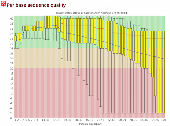
In this plot:

• the red line is the median quality score;
• the yellow box represents the interquartile range;
• the whiskers show a wider spread of reads;
• the blue line represents the mean quality;
• green, orange, and red background bands are FastQC’s broad good, warning, and poor regions.

A decline toward the $3^{\prime }$ end is common. The key question is whether the low-quality portion is substantial enough to affect the retained reads and whether it differs sharply between samples.

For an initial portfolio policy, you might write:

Per-base quality criterion: After any documented trimming, no retained read-position group should have a median quality below $Q20$. A pronounced low-quality tail in raw reads triggers trimming assessment, not automatic trimming. Any sample with substantially poorer quality than the rest of its cohort is reviewed individually.

This is a review trigger, not a license to remove inconvenient samples. In the next RNA-seq QC module, you will refine trimming decisions using adapter content, sequence overrepresentation, and the location of the quality decline.

Use mapping and library metrics in context

For a well-annotated human or mouse reference, unique mapping rate is a useful starting criterion. The HBC Training MultiQC guidance suggests at least $75\%$ uniquely mapped reads as a good-quality benchmark and advises investigation once rates drop below $60\%$. These values are less appropriate for a poorly assembled organism, incomplete annotation, contamination-prone samples, or an assay whose reads are not expected to map primarily to the reference genome.

A practical initial policy for a human or mouse, bulk, poly(A)-selected project could look like this:

Metric	Pass	Warning / review	Hold	Interpretation
Unique genomic mapping	$\ge 75\%$	$60\%$ to less than $75\%$	$<60\%$	Check reference compatibility, contamination, rRNA content, read quality, and library type.
Exonic reads	$>60\%$	Lower than expected for the protocol	Very high intergenic fraction, especially $>30\%$	Poly(A)-selected human or mouse libraries should generally be exonic; protocol and annotation matter.
GC content	Similar cohort-level profile	One sample visibly displaced from peers	Strong unexplained separation paired with other QC concerns	Evaluate together with duplication, mapping, and source metadata.
Duplication	Comparable across similar samples	Large unexplained between-sample difference	Do not set a universal failure threshold	RNA-seq duplicates can reflect genuinely abundant transcripts, not only PCR artefacts.
$5^{\prime }$ to $3^{\prime }$ coverage bias	Approximately even coverage	Bias approaching the reported review range	Strong bias with degradation or preparation evidence	Investigate RNA integrity and library preparation.

Do not treat the final column as a generic checklist to copy without modification. Write the organism, library protocol, mapper or quantifier, reference release, and rationale alongside your thresholds.

---

Differential-expression acceptance: can the comparison support the claim?

A trustworthy DE result begins before DESeq2 runs. Your analysis needs valid inputs, a defined comparison, and an audit trail for every gene excluded or flagged.

The inputs and question must agree

Before model fitting, require all of the following:

1. Counts are raw, non-negative integers.
   DESeq2 expects estimated counts rather than TPM, FPKM, log-transformed values, or manually normalized values.

2. Every count column has exactly one metadata row.
   The matching sample identifiers must be unique. This is a pass-or-hold criterion: there is no acceptable partial match.

3. The design and contrast are written in biological language first.
   For example: “Which genes differ between treatment and vehicle at 24 hours?” Then record the DESeq2 contrast direction so that a positive log2 fold change has an unambiguous meaning.

4. Replication represents independent biological units.
   Technical lanes or resequencing runs cannot be counted as biological replicates. For a portfolio comparison, set a minimum of three independent biological replicates per group as a baseline operational requirement. More replication is preferable, and three does not guarantee adequate power.

5. The comparison is estimable.
   Each condition must have samples, and a condition must not be completely inseparable from a known batch variable. A model cannot distinguish treatment from batch if every treatment sample came from one batch and every control came from another.

A useful criterion is therefore:

Design acceptance criterion: The sample sheet has one unique row per count-matrix column; each comparison group has at least three independent biological replicates; all levels included in the model are represented as documented; and no stated covariate is completely confounded with condition.

You will examine confounding formally in the experimental-design module. For now, make it visible and refuse to call a result “trustworthy” if the metadata cannot support the stated comparison.

Low-count filtering must be predeclared

Genes with almost no counts in the study provide little statistical information and increase the multiple-testing burden. A reasonable prefilter uses only count abundance and group size, never the observed p-values or fold changes.

For a two-group design with three samples per group, a documented rule might be:

$$\text{retain gene if it has at least 10 counts in at least 3 samples}$$

In R, that rule is commonly expressed as:

smallest_group_n <- min(table(colData(dds)$condition))

keep <- rowSums(counts(dds) >= 10) >= smallest_group_n
dds <- dds[keep, ]

The exact threshold may differ for your experiment, but the policy should be frozen before examining which genes are significant. Record:

• total genes before filtering;
• genes retained;
• genes removed;
• count threshold;
• smallest group size;
• the reason for choosing the rule.

DESeq2 also performs independent filtering by default when producing results. This is distinct from a project-level prefilter: it uses mean normalized counts to improve the number of detectable genes at the specified false-discovery-rate level, and it records genes that receive NA adjusted p-values because they did not pass the filter.

Sample relationships are evidence, not a cosmetic figure

A PCA plot or sample-distance heatmap is not expected to show one perfect cluster per condition. Biological heterogeneity, time, sex, genotype, tissue composition, and batch can all contribute meaningful variation.

Your acceptance policy should require that:

• all samples appear in sample-level QC plots;
• the metadata used to colour or annotate plots include condition and known technical variables;
• extreme or isolated samples are investigated;
• no sample is removed solely because it weakens a preferred biological narrative;
• any removal has independent technical or biological justification and is documented.

To make “investigate outliers” operational, define a review trigger. For example:

Sample-outlier review criterion: Flag a sample when its median variance-stabilized distance to all other samples exceeds the cohort median by more than three median absolute deviations. Review raw-read QC, mapping, library metrics, metadata, and experimental notes. A flag triggers review; it does not automatically justify exclusion.

This threshold is a screening device, not a claim that the sample is erroneous. With small RNA-seq studies, judgment must incorporate the full evidence.

Interpret Cook’s distance and NA values correctly

DESeq2 calculates Cook’s distance to detect whether an individual sample count exerts unusually large influence on a gene’s fitted model. With sufficient replication, DESeq2 flags genes affected by such outliers by setting their p-values and adjusted p-values to NA.

That is an important feature of a trustworthy result table, not an error to bypass by replacing NA values with zeros or filtering them away without explanation.

A concise Cook’s-distance criterion can be:

Influential-count criterion: Retain DESeq2’s default Cook’s-distance handling. Report the number and proportion of genes with p-values or adjusted p-values set to NA because of outlier filtering. If flagged genes are concentrated in one sample, place the analysis on hold for sample-level review.

The criterion does not need to demand zero outliers. Biological datasets can have genuine rare events and isolated high counts. What is unacceptable is an unexplained pattern that is hidden from the final report.

---

Define “differentially expressed” before looking at the answer

A common reporting rule is:

$$\text{adjusted p-value}\le 0.05$$

and

$$\left|{\log }_2(\text{fold change})\right|\ge 1$$

The first condition controls the false discovery rate at the chosen level; the second applies a practical effect-size threshold of at least a twofold change in either direction.

For a portfolio project, this is a reasonable default if you state it in advance. Your acceptance document should also state:

• which contrast was tested;
• which group is the reference level;
• whether the reported log2 fold changes are shrunken for ranking and visualization;
• the chosen FDR level;
• the chosen effect-size threshold;
• the number of genes tested;
• the number filtered for low counts;
• the number with NA p-values or adjusted p-values, with reasons;
• the number passing the final reporting rule.

Crucially, a trustworthy analysis does not require a minimum number of significant genes. A result with zero genes meeting the threshold can be scientifically valid. A result with thousands of genes can be valid too, but it deserves closer review for experimental-scale effects, batch differences, or an unexpectedly broad response.

Use wording such as:

“Genes were reported as differentially expressed when adjusted p-value was at most $0.05$ and absolute log2 fold change was at least $1$. This criterion was chosen before inspection of gene-level results. Genes excluded by low-count filtering and genes with NA adjusted p-values were retained in the full results table and summarized separately.”

That is much stronger than writing “significant genes were selected” after observing the data.

---

Build your project’s acceptance-criteria file

Create:

docs/acceptance_criteria.md

Use a table with a concrete owner, evidence location, and action. Adapt the placeholder paths and thresholds to your project.

ID	Stage	Metric and rule	Statuses	Evidence	Action if not accepted
RUN-01	Input	Expected sample IDs equal raw-input manifest IDs.	Pass or hold	metadata/asset_inventory.tsv	Stop and reconcile missing, extra, or renamed samples.
RUN-02	Tracking	Count-matrix columns equal metadata IDs, with no duplicates.	Pass or hold	Validation output	Stop before DESeq2 dataset construction.
QC-01	Read quality	Retained read positions have median quality at least $Q20$.	Pass, review, hold	FastQC and MultiQC	Review read-end decline and adapter evidence.
QC-02	Mapping	Unique genomic mapping at least $75\%$; review below $75\%$; hold below $60\%$.	Pass, review, hold	MultiQC mapping summary	Check reference, assay, contamination, and library characteristics.
QC-03	Cohort consistency	Major GC, duplication, and coverage differences are reviewed across samples.	Pass or review	MultiQC plots	Check library preparation, degradation, and metadata.
DE-01	Design	At least three independent biological replicates per compared group; metadata and count columns match exactly.	Pass or hold	Sample sheet and validation log	Stop and correct design or redefine the comparison.
DE-02	Filtering	Keep genes with at least 10 counts in at least the smallest-group sample count.	Pass or hold	Analysis configuration and filtering summary	Do not inspect DE results until rule is set.
DE-03	Sample QC	Every sample is assessed by transformed-count PCA and sample-distance analysis.	Pass, review, hold	PCA and distance heatmap	Investigate flagged samples; document any exclusion.
DE-04	Outliers	Cook’s-distance-flagged genes are counted and reported; sample-level concentration is investigated.	Pass, review, hold	DESeq2 summary and Cook’s plot	Hold interpretation if a sample-level issue is unresolved.
DE-05	Reporting	Final DE label uses adjusted p-value at most $0.05$ and absolute log2 fold change at least $1$.	Pass	Full and filtered DE tables	Export both tables and report gene counts transparently.

Add a short scope statement above the table, for example:

These criteria apply to paired-end, poly(A)-selected bulk RNA-seq libraries from a human or mouse study analyzed against the documented genome and annotation release. Mapping thresholds are review triggers, not universal biological quality standards.

Finally, create a run-specific record, such as:

results/run_2026_03_15/acceptance_summary.md

This file should state each criterion’s observed value, status, decision, and any exception. Your future automation can generate much of this summary, but writing it manually once will clarify what the pipeline must eventually validate.

---

Key takeaways

A successful RNA-seq pipeline run and a trustworthy differential-expression result are related but different claims.

• Run acceptance verifies complete inputs, exact sample tracking, successful commands, traceable references, and interpretable technical QC.
• DE acceptance verifies a valid count matrix and metadata mapping, independent replication, a defined comparison, predeclared filtering, sample-level diagnostics, and transparent outlier handling.
• A FastQC or MultiQC warning is a prompt for investigation, not an automatic failure or an automatic trimming decision.
• Mapping-rate thresholds depend on organism and reference quality; document their scope rather than treating them as universal.
• A DE threshold such as adjusted p-value at most $0.05$ plus absolute log2 fold change at least $1$ is defensible only when selected before examining results.
• Zero significant genes is not a failed analysis. Missing samples, mismatched identifiers, confounded metadata, or unreviewed sample outliers are much more serious threats to trustworthiness.

Next, you will use these criteria and the earlier inventory to organize the repository so code, configuration, documentation, tests, and generated outputs have clear, separate locations.