Sample and Metadata Inventory Design

Hello. In the previous lesson, you mapped the path from raw reads to differential expression and functional interpretation. A diagram tells a reviewer how information moves through the project. This lesson creates the companion artifact that tells them what each item actually is, where it belongs, and how it relates to a biological sample.

By the end, you will have a practical inventory for your RNA-seq project that separates raw data, derived data, code, and results, while linking files back to consistent sample metadata. This is the basis for reproducibility, debugging, and a portfolio repository that another analyst can understand quickly.

---

An inventory is not just a file list

A directory listing such as this is not yet an inventory:

sample1_R1.fastq.gz
sample1_R2.fastq.gz
counts_final.csv
DESeq2_final.R
final_results.csv
plot_new.png

It gives no reliable answers to important questions:

• Is sample1 a biological sample, a sequencing library, or a technical repeat?
• Was counts_final.csv generated from raw counts, normalized counts, or transformed values?
• Which script produced final_results.csv?
• Does plot_new.png show a QC diagnostic, a PCA, or a final biological result?
• Can the raw files be recovered if they are not stored locally?
• Which metadata values define the differential-expression comparison?

A useful inventory establishes identity, role, location, and provenance for each meaningful asset. It should allow a reviewer—and future you—to trace a result back to its inputs without guessing from filenames.

The central distinction is based on a file’s role, not merely its extension.

Class	Definition	RNA-seq examples	Can it normally be regenerated?
Raw data	Original data received from a sequencing facility or public repository	FASTQ.gz read files, vendor run sheet, original sample submission sheet	Not from your pipeline; preserve unchanged
Derived data	Intermediate data generated during processing	trimmed FASTQ files, BAM files, quant.sf, featureCounts matrix, DESeq2-normalized counts	Yes, if raw data, references, configuration, and code are available
Code	Human-written instructions that perform or validate analysis	Bash scripts, R scripts, Quarto source, test scripts	Maintained and version-controlled rather than regenerated
Results	Interpretable outputs used to support a conclusion or communicate findings	QC summary, PCA figure, DESeq2 contrast table, volcano plot, enrichment table, final report	Yes, but should be retained as documented evidence

There is also a small but important fifth group: supporting artifacts. These include sample metadata, configuration files, reference-version records, checksums, software environments, logs, and documentation. They may not be primary analysis data or results, but without them a run is difficult to reproduce or audit.

The dividing line between derived data and results is especially useful:

• A gene-count matrix is derived data: it is a computational input to statistical analysis.
• A DESeq2 result table is a result: it contains inferential output for a specified comparison.
• A FastQC report is a result in the sense of QC evidence, even though it does not answer the biological question directly.
• A BAM file is derived data; an alignment summary or MultiQC report is QC evidence about it.

---

Metadata gives the files biological meaning

Sequence reads are only technically identifiable until they are linked to metadata. A FASTQ filename tells you that reads exist; metadata tells you what was sequenced, under which condition, with what quality, and how it should enter the model.

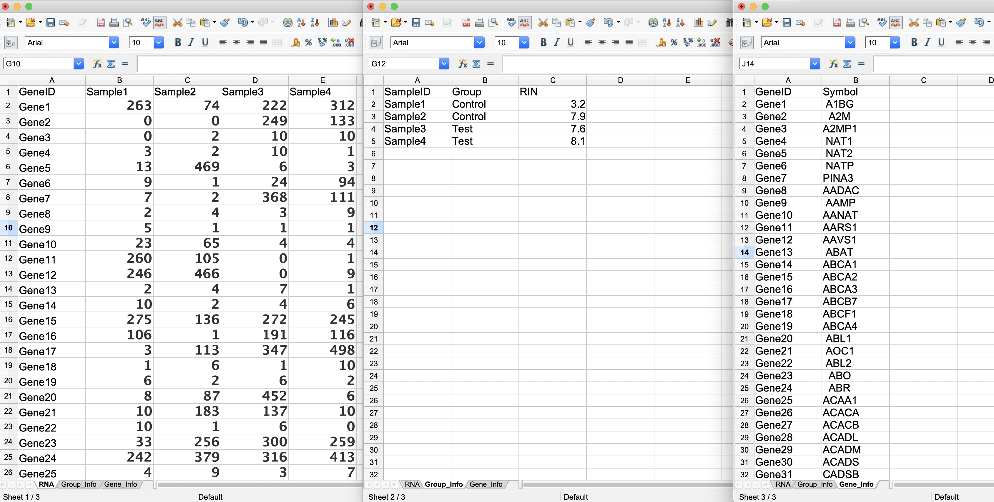
In this image, the count matrix is derived data. The table with Group and RIN is sample metadata. The gene-ID mapping is annotation metadata. Treating these as separate, linked tables prevents a common RNA-seq mistake: putting experimental information into ad hoc count-column names such as Control_RIN7.9_Sample2.

For a DESeq2 analysis, a metadata table usually has one row per analysis unit represented by one count-matrix column. In many bulk RNA-seq projects, that unit is a sequenced library. Do not assume that a short filename prefix identifies the biological sample unambiguously: one biological specimen can have multiple libraries or runs.

The ENA conceptual model makes the distinction clearer.

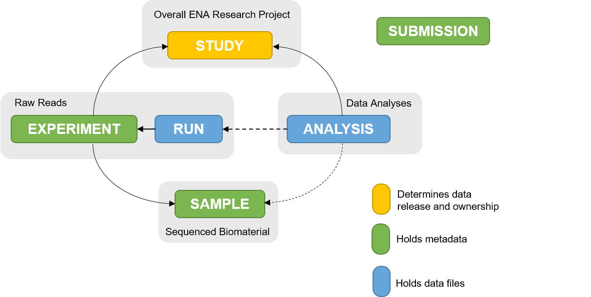
For your project, you do not need to reproduce the full ENA schema. But you should preserve the core identities:

• study_id: the dataset or project identifier, such as a GEO series or SRA BioProject.
• biological_sample_id: the original biological material.
• library_id: the prepared sequencing library, if known.
• run_id: a sequencing run or public accession, if applicable.
• sample_id: the stable identifier used in your analysis metadata and count matrix.

If a public dataset does not expose every identifier, record the identifiers it does provide and state what is unknown. Honest incompleteness is safer than inventing a one-to-one relationship between FASTQ files and biological samples.

---

Use two linked inventories, not one overloaded spreadsheet

For a portfolio project, create two primary tab-separated files in a location such as metadata/. TSV is convenient because it is plain text, Git-friendly, and easy to import into R. CSV is equally acceptable if you use it consistently.

1. sample_metadata.tsv records attributes of samples or libraries.
2. asset_inventory.tsv records files, directories, accessions, scripts, and results.

A separate metadata_dictionary.md defines every column, permitted values, units, and missing-value conventions. This prevents silent inconsistencies such as control, Control, CTRL, and untreated being used for the same condition.

1. Sample metadata: one row per analysis sample

Below is a compact template. Replace the example values with values appropriate to your project.

sample_id	biological_sample_id	library_id	condition	batch	rin	organism	assay	read_layout
S01	BIO_01	LIB_01	control	batch_1	8.2	Homo_sapiens	bulk_RNA_seq	paired
S02	BIO_02	LIB_02	control	batch_1	7.9	Homo_sapiens	bulk_RNA_seq	paired
S03	BIO_03	LIB_03	treatment	batch_1	8.1	Homo_sapiens	bulk_RNA_seq	paired
S04	BIO_04	LIB_04	treatment	batch_1	7.6	Homo_sapiens	bulk_RNA_seq	paired

Use a stable sample_id that matches the count-matrix column names exactly. This is the join key that will later connect your metadata to DESeq2.

A few design decisions matter:

• Use condition, not vague labels such as group or type.
• Keep continuous variables such as RIN in their own numeric column.
• Keep batch information in its own column even if it is not currently included in the model.
• Use consistent controlled values such as control and treatment; do not alternate capitalization.
• Use NA only when it has a documented meaning. Do not use NA, blank cells, unknown, and - interchangeably.
• Do not store sensitive participant information in a public repository. Use de-identified IDs and record access restrictions where needed.

Avoid encoding several variables in one field:

Bad:  treatment_batch2_female
Better: condition = treatment; batch = batch_2; sex = female

The second form can be filtered, checked, and included in a statistical design when scientifically justified.

2. Asset inventory: one row per file or logical asset

The asset inventory records what the asset is, rather than trying to infer its purpose from its directory or filename. For paired-end reads, one row per physical FASTQ file is the most auditable approach.

asset_id	asset_class	asset_type	sample_id	relative_path_or_accession	producer_or_source	status	checksum_note
raw_S01_R1	raw_data	fastq_read1	S01	data/raw/S01_R1.fastq.gz	ENA:ERR000001	available	record_sha256
raw_S01_R2	raw_data	fastq_read2	S01	data/raw/S01_R2.fastq.gz	ENA:ERR000001	available	record_sha256
qc_S01	results	fastqc_report	S01	results/qc/fastqc/S01_fastqc.html	FastQC	vetted	not_applicable
bam_S01	derived_data	sorted_bam	S01	data/derived/alignment/S01.sorted.bam	STAR	vetted	record_sha256
counts_v1	derived_data	gene_count_matrix	NA	data/derived/counts/gene_counts.tsv	featureCounts	vetted	record_sha256
deseq_script	code	R_analysis	NA	scripts/04_deseq2.R	author	active	Git_tracked
de_treat_vs_ctrl	results	DESeq2_result_table	NA	results/differential_expression/treatment_vs_control.tsv	DESeq2	vetted	Git_tracked
pca_plot	results	QC_figure	NA	results/qc/pca_vst.png	R_script	active	Git_tracked

This is a starting structure, not an immutable standard. The key columns serve distinct purposes:

Column	Purpose
asset_id	A stable unique identifier for this asset
asset_class	Controlled category: raw_data, derived_data, code, results, or supporting
asset_type	Specific kind of object, such as fastq_read1, count_matrix, or DESeq2_result_table
sample_id	The related analysis sample; use NA for project-level assets
relative_path_or_accession	A project-relative location or public accession—not a personal absolute path
producer_or_source	Tool, script, repository, sequencing facility, or public database that supplied it
status	A controlled review state, such as available, active, vetted, deprecated, or missing
checksum_note	Whether and where integrity information is recorded

Do not force an asset into the wrong class simply to fill one of the four required categories. Examples of supporting assets include:

metadata/sample_metadata.tsv
config/analysis_parameters.yaml
references/reference_manifest.tsv
environment/environment.yml
logs/run_2026-04-18.log
docs/metadata_dictionary.md

These items make the relationship among raw data, code, derived data, and results inspectable.

---

Establish lineage without making a spreadsheet unreadable

An inventory should make it possible to reconstruct provenance, but it does not need to put an entire workflow graph into one cell.

For simple assets, producer_or_source plus the project-relative path is often enough:

• S01.sorted.bam was produced by STAR.
• gene_counts.tsv was produced by featureCounts.
• treatment_vs_control.tsv was produced by the DESeq2 script.

When the project grows, add a third table, asset_lineage.tsv, with one relationship per row:

child_asset_id	parent_asset_id	relationship
bam_S01	raw_S01_R1	derived_from
bam_S01	raw_S01_R2	derived_from
counts_v1	bam_S01	derived_from
de_treat_vs_ctrl	counts_v1	analyzed_from

This keeps each cell atomic and makes it possible to track multiple parents cleanly. It also mirrors the logic of the data-flow diagram from the previous lesson: each data product has named upstream inputs and a named process that generated it.

For public datasets, an accession can be more useful than a local copy. For example, if FASTQ files are too large for your repository, record:

• the BioProject, GEO, SRA, or ENA accession;
• the exact run accessions used;
• download date, if relevant;
• checksum or file-size verification status;
• licensing or access restrictions;
• the script or command that retrieves the data.

Never upload large raw FASTQ, BAM, or generated intermediate files to Git merely to make the repository look complete. A clear inventory plus retrieval instructions is stronger evidence of professional data management.

---

Build your project inventory

Create the following three files now:

metadata/sample_metadata.tsv
metadata/asset_inventory.tsv
docs/metadata_dictionary.md

This is a lightweight working layout, not the final repository architecture; you will formalize repository organization later in the module.

Step 1: Start from the DESeq2 input

Find the count matrix that your existing DESeq2 analysis uses. Record it as derived_data with asset_type = gene_count_matrix.

Then answer these questions in the inventory:

• Which tool created it: featureCounts, htseq-count, tximport, or another method?
• Which annotation or transcript-to-gene mapping did it depend on?
• Which sample IDs form its column names?
• Is it raw integer count data, or has it been normalized or transformed?

For DESeq2, the modeling input should normally be raw integer-like counts or an appropriate imported count representation—not TPM, FPKM, or a log-transformed matrix. Record the actual form rather than calling every table “counts.”

Step 2: Add each sample and raw-read pair

For every count-matrix sample column:

1. Create one metadata row using the exact sample_id.
2. Add one asset-inventory row for read 1 and one for read 2 if the assay is paired-end.
3. If reads came from a public source, record the accession even if you also retain a local path.
4. Mark files as raw_data; do not classify copied or downloaded raw reads as derived just because you downloaded them yourself.

If your data are single-end, record one FASTQ asset per sample and use read_layout = single.

Step 3: Add meaningful derived assets

You do not need to list every temporary file. Add assets that are inputs to major stages, checkpoints in the workflow, or necessary for inspection:

• post-trimming FASTQ files, if trimming was performed;
• alignment BAM files or transcript-quantification directories;
• count matrix;
• gene annotation mapping used for result annotation;
• transformed expression matrix, if saved and reused;
• MultiQC summary, if created.

A practical rule is: include an intermediate if deleting it would make the pipeline difficult to resume, audit, or explain.

Step 4: Add code and results

List each analysis entry point rather than every small helper immediately:

• main Bash pipeline script;
• R script that constructs the DESeq2 dataset and generates results;
• functional-analysis script or notebook;
• report source file;
• configuration file.

Then list the results you would show in a portfolio review:

• QC summary report;
• PCA or sample-distance figure;
• annotated DE result table for the stated contrast;
• MA plot and volcano plot, if used;
• enrichment result table and figure;
• final rendered report.

Use names that reflect the comparison. treatment_vs_control.tsv is more informative than final_DE_results.tsv.

---

Perform three fast consistency checks

Before treating the inventory as complete, perform these checks manually or in R.

Sample coverage

Every sample_id in the count matrix should appear once and only once in sample_metadata.tsv. Every sample should have the expected raw-read assets, unless you document why not.

Identifier consistency

The identifiers must match exactly across:

• count-matrix columns;
• sample_metadata.tsv;
• FASTQ asset rows;
• quantification or BAM asset rows;
• sample names in QC reports.

Sample_01, sample01, and S01 may look equivalent to a human, but they are distinct strings to R and Bash.

Category sanity

Ask one question for every item:

Is this original input, a reproducible intermediate, human-authored instructions, an interpretable output, or supporting evidence?

If you cannot answer clearly, improve the asset_type, path, documentation, or filename. Ambiguous assets tend to be the ones that later cause accidental use of normalized data as counts, stale results after reruns, or confusion about which script produced a figure.

---

Key takeaways

A job-ready RNA-seq project should contain a deliberate inventory, not an undocumented pile of files.

• Raw data are original sequencing inputs and should remain unchanged.
• Derived data are reproducible intermediates, including alignments, quantifications, and count matrices.
• Code contains the version-controlled instructions that perform analysis.
• Results are the reports, figures, and statistical tables used to evaluate quality and support conclusions.
• Sample metadata gives files biological and experimental meaning; it must use stable identifiers that match the count matrix.
• A data dictionary and controlled values prevent small metadata inconsistencies from becoming analytical errors.

In the next lesson, you will inspect the assumptions hidden in filenames, directory structures, and metadata—exactly the assumptions this inventory has begun to expose.