Pipeline Data-Flow and Quality Checks

Good to continue from the project-scope statement you drafted previously. You now have the question your analysis is meant to answer; this lesson turns that statement into a second essential portfolio artifact: a data-flow diagram.

A reviewer should be able to look at your diagram and understand what enters each pipeline stage, what that stage produces, and what evidence you use to decide whether the output is trustworthy. This is more informative than a list of tools, and it gives you a practical map for debugging and documenting your Bash pipeline.

By the end of this lesson, you will have a draft workflow diagram for your own repository, covering raw reads through differential expression and functional interpretation.

---

A pipeline diagram is an evidence map

A weak workflow diagram says:

FastQC, trimming, alignment, featureCounts, DESeq2.

That is a tool list. It does not show whether the analysis can actually be reproduced or audited.

A useful data-flow diagram treats every stage as a small contract:

Part of the contract	Question it answers	Example
Inputs	What must exist before this stage runs?	Raw FASTQ files, transcriptome index, sample sheet
Processing	What operation is performed?	Read QC, pseudoalignment, counting, DESeq2 model fitting
Outputs	What new data or report is created?	quant.sf, count matrix, DE result table
Quality checks	What evidence tells us whether the output is credible?	FastQC report, mapping rate, count-assignment summary, PCA
Decision or gate	What changes if the check indicates a problem?	Trim only if evidence supports it; stop if sample labels disagree

The distinction between an output and a quality check matters. A FASTQ file is data passed into the next stage. A FastQC HTML report is evidence about that FASTQ file. A BAM file can proceed to counting, while alignment statistics and gene-body coverage reports help you judge whether that BAM file is suitable for counting.

The supplied workflow image demonstrates this separation well: the main analysis path proceeds from reads to quantification, differential expression, and functional analysis, while QC appears as a parallel evidence stream.

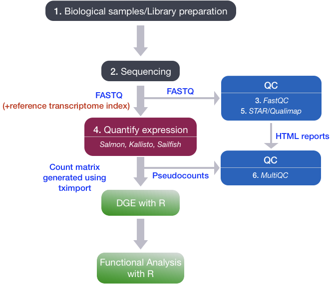
Do not copy this diagram blindly. It shows one valid Salmon-based route. Your portfolio diagram must reflect the tools and files in your current project.

---

First choose the route your project actually follows

Bulk RNA-seq pipelines usually reach gene-level count inputs through one of two broad routes.

Route A: transcriptome quantification

Tools such as Salmon or Kallisto compare reads with a reference transcriptome index and produce transcript-level abundance files, often named quant.sf. A tool such as tximport then combines sample-level quantification files and transcript-to-gene information into gene-level inputs appropriate for downstream differential-expression analysis.

Typical evidence includes:

• mapping or assignment rate;
• inferred versus expected library type;
• number of reads processed;
• reference/index version;
• consistency of quantification files across samples.

Route B: genome alignment followed by read counting

A splice-aware aligner such as STAR, HISAT2, or another aligner maps reads to a reference genome, producing alignment files such as sorted BAM files. A counting tool, for example featureCounts, uses the corresponding GTF/GFF annotation to assign aligned reads to genes and generate a count matrix.

Typical evidence includes:

• overall and unique mapping rates;
• multimapping, mismatch, and splice-junction metrics;
• strandedness consistency;
• assignment and unassignment categories from the counting summary;
• compatibility of genome, annotation, and aligner index versions.

The curated tutorial illustrates this second route from FASTQ files through quality control, trimming where justified, genome alignment, BAM files, feature-level counting, and a final count matrix.

A diagram should show one route as your primary path. Do not draw Salmon, STAR, and featureCounts consecutively unless your project genuinely runs all three for distinct stated purposes. Combining alternative workflows into one apparent sequence makes your project look conceptually confused.

---

The minimum complete workflow

The following model uses a Salmon and tximport route because it corresponds to the supplied workflow image. It also makes visible the metadata, reference, configuration, and QC artifacts that are often omitted from beginner diagrams.

Read this diagram from top to bottom, but do not interpret every connecting line as a shell command. Some connections represent data passed forward, while dotted lines represent QC evidence reviewed before choosing an action.

For example:

• The first FastQC report does not automatically trim reads. It provides evidence for deciding whether trimming is warranted.
• The transcriptome index is a required reference input to quantification, even though it is not sample data.
• The sample metadata is not ordinarily an input to Salmon itself, but it is essential when constructing the differential-expression model.
• Differential expression produces both a results table and diagnostic evidence. A statistically generated results table is not automatically biologically trustworthy if PCA, size factors, or sample labels reveal a problem.

If your pipeline uses genome alignment and featureCounts, replace the Transcript quantification and Import and summarize to genes section with the following logical stages:

Stage	Inputs	Main output	QC evidence to show
Genome alignment	Analysis FASTQ files, genome index, alignment settings	SAM/BAM alignments and aligner log	Mapping rate, unique mapping, multimapping, mismatches, splice junctions
BAM processing	BAM file, processing settings	Sorted and indexed BAM file	File integrity, sort order, index presence, read-pair handling
Gene-level counting	BAM files, matching GTF/GFF annotation, strand setting	Raw gene count matrix and count summary	Assigned reads, unassigned categories, annotation compatibility
Matrix validation	Count matrix, sample metadata	Validated DESeq2 input	Matrix dimensions, sample order, duplicate identifiers, library sizes

The key rule is simple: the diagram must reflect the route that generated the count input you actually supplied to DESeq2.

---

Name artifacts, not just stages

A workflow diagram becomes much more useful when its labels name actual file classes. Compare these two labels:

• “Alignment”
• “Sorted, indexed BAM files plus Log.final.out”

The second label tells a reviewer what they should expect to find in the repository or output directory.

Use names that are specific enough to inspect but general enough to avoid tying the diagram to a single sample. For example:

Pipeline stage	Input artifacts	Output artifacts	QC artifact or check
Raw-read QC	*.fastq.gz files	FastQC HTML and ZIP reports	Per-base quality, adapter content, GC distribution, overrepresented sequences
Optional trimming	Raw FASTQ files and trimming settings	Trimmed FASTQ files	Read retention; post-trimming FastQC comparison
Quantification	Analysis FASTQ files, index, configuration	One quantification directory per sample	Mapping/assignment rate; library-type evidence
Alignment route only	Analysis FASTQ files, genome index, annotation	Sorted BAM and index	Alignment summary, mismatch and splice metrics
Read counting or import	BAM plus GTF/GFF, or quantification files plus transcript-gene map	Gene-level count input	Assignment summary; gene IDs; sample-column consistency
Differential expression	Count input, metadata, design specification	Annotated gene-level results	PCA/sample distance, size factors, model diagnostics
Functional analysis	Result table, tested-gene universe, annotations	ORA/GSEA tables and figures	Identifier mapping rate; pathway redundancy; leading genes

Notice that trimming is optional, while raw-read QC is not. A diagram that always includes trimming silently communicates that it happens by default, rather than in response to evidence. That is an analytical choice you will audit more deeply in Module 6.

Also, avoid vague labels such as “clean data,” “final output,” or “analysis results.” A recruiter or interviewer cannot inspect those claims. Labels such as “post-trim paired FASTQ files,” “gene count matrix,” and “DESeq2 contrast table” can be verified.

---

Quality control should be connected to decisions

QC is not a decorative side panel. Every important check should answer a practical question.

QC evidence	Decision it supports
Poor base quality or adapter contamination in raw-read reports	Whether trimming is justified and what problem it should address
Post-trimming read retention and FastQC comparison	Whether trimming removed the expected issue without making reads unusably short
Alignment or quantification metrics	Whether reads plausibly match the stated organism, reference, and assay
Read-count assignment summary	Whether the annotation, strand setting, and alignment assumptions are plausible
Count matrix dimensions and sample names	Whether every expected sample is present exactly once and correctly labeled
Library-size profile, PCA, and sample-distance diagnostics	Whether samples show unexpected technical separation or potential outliers
Identifier mapping in enrichment	Whether pathway claims are based on a known and adequate portion of the tested genes

At this point, do not try to set universal numeric pass/fail thresholds. Those will be developed later as project-specific acceptance criteria. For now, ensure the diagram shows that the checks exist, states the evidence generated, and makes clear which stage that evidence evaluates.

---

Build your repository version now

Create docs/workflow.md in your project repository. Add a short opening statement such as:

This diagram describes the data flow for the primary bulk RNA-seq analysis. It documents the actual processing route used to generate the count input for DESeq2 and the QC evidence reviewed at each stage.

Then copy the Mermaid model into the file and edit it using your real project details.

Work systematically:

1. Trace backward from the DESeq2 input. Identify the exact matrix or tximport object used in your existing analysis, then identify the command and upstream files that generated it.
2. Choose one quantification route. Keep either the Salmon-style section or the align-and-count section as the primary route.
3. Replace generic references. State the actual reference type used: for example, a transcriptome index, or a genome assembly and GTF annotation. Include version or release identifiers where you know them.
4. Add QC sidecars. For every major data stage, name the report, log, or validation check that evaluates it.
5. Represent metadata explicitly. Draw sample metadata into differential expression, because conditions, batches, pairing, and reference levels are not encoded reliably in a count matrix alone.
6. Mark unknown details honestly. Use a label such as “reference release to verify” rather than guessing from an old filename or script default.

Before committing, use this completeness review:

• The diagram starts with the raw sequencing data that your pipeline actually receives.
• Every central stage has at least one input and one named output.
• QC reports are attached to the stage that produced or evaluated them.
• The chosen quantification route matches the files used by DESeq2.
• The diagram includes sample metadata and reference resources, not only FASTQ files and tools.
• Functional analysis is shown as downstream interpretation, not as proof that a pathway is causally altered.
• A reader can locate the expected artifacts from the labels alone.

This document is not merely presentation material. When a run fails, the diagram gives you a structured debugging sequence: identify the missing or implausible output, locate its upstream inputs and QC evidence, then inspect the relevant command, configuration, and log.

---

Key takeaways

A job-ready RNA-seq workflow diagram shows more than software names. It links:

• inputs such as FASTQ files, metadata, references, and configuration;
• processing stages that transform those inputs;
• inspectable outputs such as reports, BAM files, quantification files, count matrices, and result tables; and
• quality checks that support decisions rather than merely decorate the workflow.

Use one clear primary route: transcriptome quantification plus tximport, or genome alignment plus gene counting. Keep QC as a parallel evidence stream, and make metadata visible where it becomes essential to the statistical model.

Next, you will build a sample-and-metadata inventory that distinguishes raw data, derived data, code, and results. That inventory will give the diagram concrete file locations and make its assumptions easier to inspect.