Estimating Throughput, Storage Growth, and Bandwidth Needs

Welcome back. The container diagram from the previous lesson established the pilot’s operational boundaries: a Telemetry Connector collects Microsoft Entra ID events, a durable event log separates ingestion from detection, a Detection Worker creates alert summaries, PostgreSQL holds investigation state, and object storage retains evidence.

This lesson tests whether that design is plausible at scale. You will turn a stated workload into three kinds of numbers:

• throughput: events or requests per second that each path must sustain;
• storage growth: bytes per day, retention footprint, replicas, and operating reserve;
• bandwidth: byte rates over external, service, and broker-network links.

The goal is not fake precision. It is a transparent model with explicit assumptions, rounded conservatively, that exposes the next engineering questions.

---

Capacity planning is an assumptions contract

A capacity model has two parts:

1. Inputs that product, security, engineering, and operations can challenge.
2. Derived values that follow mechanically from those inputs.

Do not begin with an instance type, number of Kafka brokers, or a database SKU. Those are decisions made after you know the workload to be served.

The capacity-planning flowchart below captures the right broad order: workload assumptions drive storage, network, and compute estimates; the most demanding constraint, plus fault tolerance and headroom, informs the eventual broker or node count.

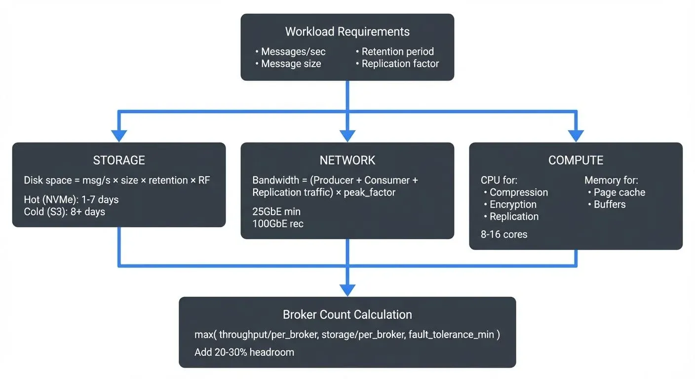
For the Tenant Behavioral Detection Platform, use the following planning scenario. These are deliberately assumptions for a pilot, not claims about Microsoft Entra ID or an eventual customer base.

Assumption	Value	Why it matters
Tenants	$2,000$	Establishes the multi-tenant population.
Active identities per tenant	$20,000$	Creates a total monitored identity population.
Security events per identity per day	$25$	Includes sign-ins and other selected audit events.
Normal peak multiplier	$4$	Models diurnal concentration and connector polling behavior.
Attack burst	$3$ times normal peak for $15$ minutes	Models an abuse or incident-driven traffic surge.
Raw source event size	$1.5$ KB	Used for external ingest and evidence archival traffic.
Normalized event size	$1.0$ KB	Used for the event log and Detection Worker path.
Durable event-log retention	$3$ days	Supports replay after processing failure.
Event-log replication factor	$3$ total copies	Protects against broker loss.
Evidence retention	$90$ days	Supports investigation and retention needs for the pilot.
Compressed evidence size	$60\%$ of raw	A planning assumption to validate with real samples.
Alert rate	$0.02\%$ of events	Supports a PostgreSQL investigation-store estimate.
Alert and investigation state	$5$ KB per alert	Includes alert metadata and associated state, before database overhead.
Investigation retention	$180$ days	A separate lifecycle from raw evidence.

Use decimal units throughout this lesson:

$$1\mathrm{KB}=1,000\mathrm{bytes}$$ $$1\mathrm{TB}=10^{12}\mathrm{bytes}$$

This avoids mixing decimal cloud-storage pricing units with binary memory units. The difference is not the important uncertainty at this stage; undocumented event size, index expansion, retry behavior, and retention policy are.

---

Derive event throughput before estimating machines

First, calculate daily event volume.

$$N_{\mathrm{identities}}=2,000\times 20,000=40,000,000$$ $$E_{\mathrm{day}}=40,000,000\times 25=1.0\times 10^{9}events/day$$

The mean event rate is therefore:

$$R_{\mathrm{average}}=\frac{1.0\times 10^9}{86,400}\approx 11,600events/s$$

A system designed only for this mean rate will fail during ordinary daily concentration. Applying the fourfold normal peak multiplier gives:

$$R_{\mathrm{normal}\mathrm{peak}}=11,600\times 4\approx 46,400events/s$$

Round up for planning:

$$R_{\mathrm{normal}\mathrm{peak}}=48,000events/s$$

During the assumed attack burst:

$$R_{\mathrm{attack}\mathrm{peak}}=48,000\times 3=144,000events/s$$

These three rates serve different purposes:

Rate	Value	Primary use
Daily average	$11,600$ events/s	Daily storage growth and long-run cost.
Normal peak	$48,000$ events/s	Routine service and network capacity.
Attack peak	$144,000$ events/s	Admission controls, durable buffering, source protection, and recovery behavior.

A frequent architecture mistake is using the peak rate for all retention calculations. That can overstate normal storage by a large factor. The reverse mistake—using the daily average to size links, queues, or processing capacity—is much more dangerous operationally.

---

Convert event rates into daily storage growth

The normalized event-log payload generated in a normal day is:

$$D_{\mathrm{normalized}\mathrm{day}}=1.0\times 10^9\times 1,000\mathrm{bytes}=1.0TB/day$$

The attack is not merely a momentary network concern. If it represents additional events rather than traffic shifted from another time of day, it increases daily data volume.

During the fifteen-minute burst, the additional event rate above the expected normal peak is:

$$144,000-48,000=96,000events/s$$ $$E_{\mathrm{attack}\mathrm{excess}}=96,000\times 900=86,400,000\mathrm{events}$$

So an attack-day volume is:

$$E_{\mathrm{attack}\mathrm{day}}=1.0\times 10^9+86.4\times 10^6=1.0864\times 10^{9}events/day$$ $$D_{\mathrm{attack}\mathrm{day}}=1.0864TB/day$$

Replication and headroom are different multipliers

For a durable event log with replication factor $3$, each retained event occupies three physical copies. Here, replication factor means total copies, not three additional replicas.

With three days of retention and one such attack burst each day:

$$S_{\mathrm{event}\log \mathrm{stored}}=1.0864TB/day\times 3\mathrm{days}\times 3=9.78\mathrm{TB}$$

The number above is stored data, not allocatable disk capacity. Operating a log cluster at nearly full disk is unsafe: partition rebalancing, a failed broker, delayed retention cleanup, and recovery all need free space.

If the operating policy is to keep utilization at or below $70\%$, calculate provisioned storage by dividing by $0.70$:

$$S_{\mathrm{event}\log \mathrm{allocated}}=\frac{9.78}{0.70}\approx 14.0\mathrm{TB}$$

This is more precise than casually “adding thirty percent.” Adding $30\%$ to used space leaves less than $30\%$ free capacity. State which convention you are using.

Evidence archive

The connector archives raw source evidence, so use the larger raw event size.

$$D_{\mathrm{raw}\mathrm{attack}\mathrm{day}}=1.0864\times 10^9\times 1.5\mathrm{KB}=1.6296TB/day$$

With a $60\%$ compression factor and ninety-day retention:

$$S_{\mathrm{evidence}\mathrm{logical}}=1.6296\times 90\times 0.60=88.0\mathrm{TB}$$

If the evidence storage budget should retain $20\%$ free capacity or equivalent cost reserve:

$$S_{\mathrm{evidence}\mathrm{budget}}=\frac{88.0}{0.80}=110\mathrm{TB}$$

For managed object storage, this is mainly a logical capacity and cost estimate. Do not multiply it by an assumed internal replication factor: the cloud provider’s durability implementation is opaque and normally already reflected in its service model and price. Do account separately for features you enable, such as object versioning, cross-region replication, legal holds, or replication to a customer-controlled archive.

PostgreSQL investigation state

The Investigation Store should not contain every raw event. It retains alert summaries, dispositions, cases, source health, and detection state. With the stated alert rate:

$$A_{\mathrm{day}}=1.0864\times 10^9\times 0.0002=217,280alerts/day$$ $$D_{\mathrm{alert}\mathrm{day}}=217,280\times 5\mathrm{KB}=1.0864GB/day$$

Assume a factor of $2$ for indexes, row versioning, and expected database overhead, then a second physical copy for high availability:

$$S_{\mathrm{postgres}\mathrm{allocated}}=\frac{1.0864GB/day\times 180\times 2\times 2}{0.70}\approx 1.12\mathrm{TB}$$

This does not include independently retained backups or point-in-time recovery logs. Those need their own retention assumptions.

The resulting storage model is intentionally separated by lifecycle and technology:

Storage responsibility	Planning footprint	What the figure means
Durable Event Log	$14.0$ TB	Physical replicated broker disk with three-day retention and $30\%$ free-space policy.
Evidence Archive	$110$ TB	Logical compressed evidence capacity and budget reserve for ninety days.
Investigation Store	$1.12$ TB	PostgreSQL data, estimated overhead, high-availability copy, and $30\%$ free-space policy.

Do not sum these and call the result “database storage.” They have different durability models, hardware constraints, query patterns, and cost structures.

The current container diagram does not include a dedicated search-index container, so do not silently invent one just because it is familiar. When the platform later adds a security-event search index, its storage model will need an explicit index expansion or compression factor in addition to retention and replica count.

---

Map the byte rates onto actual network paths

Throughput in events per second is not sufficient for network planning. Convert each path’s event rate using the size of the payload that crosses that particular boundary.

At attack peak, the connector receives raw source events:

$$B_{\mathrm{source}\mathrm{ingress}}=144,000events/s\times 1.5\mathrm{KB}=216MB/s$$ $$216MB/s\times 8=1.728Gb/s$$

It emits normalized events to the durable event log:

$$B_{\mathrm{producer}}=144,000events/s\times 1.0\mathrm{KB}=144MB/s=1.152Gb/s$$

With replication factor $3$, each leader copy produces two follower-copy transfers. The aggregate inter-broker replication rate is:

$$B_{\mathrm{replication}}=2\times 144MB/s=288MB/s=2.304Gb/s$$

The Detection Worker consumes the normalized stream once:

$$B_{\mathrm{consumer}}=144MB/s=1.152Gb/s$$

The aggregate payload through the Kafka cluster’s data paths is therefore:

$$B_{\mathrm{broker}\mathrm{aggregate}}=1.152+2.304+1.152=4.608Gb/s$$

With a $30\%$ operating margin:

$$B_{\mathrm{broker}\mathrm{planning}}=\frac{4.608}{0.70}\approx 6.58Gb/s$$

This is aggregate cluster traffic, not a per-broker NIC requirement. The per-broker rate depends on partition count, leader distribution, replica placement, consumer-group assignment, cross-zone topology, and recovery activity. Those are architectural choices that need their own model and benchmark.

The connector has a different profile:

Connector direction at attack peak	Payload rate	Planning implication
Receive from Microsoft Entra ID	$1.728$ Gb/s	Source API, TLS handling, batching, and connector ingress must withstand this rate.
Send raw evidence to archive	$1.728$ Gb/s	Evidence retention can be as network-intensive as collection.
Send normalized events to event log	$1.152$ Gb/s	This is separate from raw archival traffic.

Ignoring protocol overhead, the connector receives $1.728$ Gb/s and sends $2.880$ Gb/s concurrently. A ten-gigabit interface may look sufficient on paper, but it is not a capacity decision by itself. Measure the effect of TLS, serialization, object-store request behavior, retry storms, and uneven assignment of tenants to connector instances.

Also keep user-facing evidence retrieval separate from ingestion bandwidth. The workload brief gives no analyst-search rate, result-size distribution, or concurrent investigation count, so it cannot support a credible estimate for the Web Console and Investigation API query path yet. “Unknown” is better than a fabricated number.

---

Throughput capacity must reflect the latency objective

The Durable Event Log absorbs a burst only if its storage and network can accept the messages. It does not make detection timely by itself.

Suppose the detection path can process $96,000$ events per second during the attack. It is slower than incoming traffic, so a queue forms:

$$Q_{\mathrm{maximum}}=(144,000-96,000)\times 900=43.2\times 10^6\mathrm{events}$$

At a normalized size of one kilobyte:

$$D_{\mathrm{queue}\mathrm{maximum}}=43.2\mathrm{GB}$$

Once attack traffic returns to the $48,000$ events-per-second normal peak, the detector drains the backlog at a net rate of $48,000$ events per second. It clears the queue in fifteen minutes. The longest queueing delay is roughly:

$$\frac{43.2\times 10^6}{96,000}=450\mathrm{s}=7.5\mathrm{minutes}$$

That may be acceptable for a pilot that promises detection within ten minutes, but it would violate a five-minute end-to-end detection objective. The capacity requirement is therefore an SLO decision, not merely an infrastructure calculation.

If the chosen queue-delay budget permits this recovery behavior, $96,000$ events per second is the minimum functional processing rate. A benchmark target with $30\%$ operational headroom is:

$$R_{\mathrm{detector}\mathrm{benchmark}}=\frac{96,000}{0.70}\approx 137,000events/s$$

Similarly, the ingestion system should prove that it can accept the full attack peak with headroom:

$$R_{\mathrm{connector}\mathrm{benchmark}}=\frac{144,000}{0.70}\approx 206,000events/s$$

These are not instance counts. They are measurable acceptance and processing targets. To turn them into deployment capacity, benchmark representative production-like data and determine safe throughput per connector instance, consumer worker, and broker.

A useful benchmark should include:

• real or sanitized Entra-shaped event distributions, not only tiny synthetic JSON;
• TLS, authentication, validation, normalization, compression, and serialization;
• writes to the actual chosen event log, PostgreSQL configuration store, and evidence archive;
• p95 and p99 processing latency, not only average throughput;
• CPU, memory, disk latency, disk utilization, NIC utilization, and queue lag;
• sustained normal peak plus the attack-burst profile;
• degraded operation, such as a worker restart or broker loss.

The model tells you what to test. The benchmark reveals whether the model’s assumptions remain credible.

---

A reusable capacity-model template

For future architecture briefs, keep the arithmetic in a version-controlled spreadsheet, notebook, or small script. The core formulas are compact.

For event volume:

$$E_{\mathrm{day}}=N_{\mathrm{entities}}\times E_{\mathrm{per}\mathrm{entity}\mathrm{day}}$$ $$R_{\mathrm{average}}=\frac{E_{\mathrm{day}}}{86,400}$$ $$R_{\mathrm{peak}}=R_{\mathrm{average}}\times F_{\mathrm{peak}}$$

For a payload crossing one boundary:

$$B_{\mathrm{path}}=R_{\mathrm{peak}}\times S_{\mathrm{payload}}$$

For retained data with a storage transformation factor and total physical copies:

$$S_{\mathrm{stored}}=D_{\mathrm{day}}\times T_{\mathrm{retention}}\times F_{\mathrm{storage}}\times C_{\mathrm{copies}}$$

For allocated capacity with a target maximum utilization:

$$S_{\mathrm{allocated}}=\frac{S_{\mathrm{stored}}}{U_{\mathrm{target}}}$$

The terms must be named in the model. In particular, distinguish:

• raw versus normalized record size;
• logical object storage versus physically replicated broker disk;
• total copy count versus number of additional replicas;
• normal peak versus an attack burst;
• retained event volume versus transient consumer lag;
• throughput target versus a measured per-node capacity.

A reviewer should be able to change one assumption, such as evidence retention from ninety to one hundred eighty days, and see exactly which result changes and why.

---

Key takeaways

A capacity estimate begins with an explicit workload model, not a preferred infrastructure product. For the stated behavioral-detection pilot:

• the normal workload is approximately $1.0$ billion events per day;
• normal peak ingestion is planned at $48,000$ events per second;
• the attack scenario reaches $144,000$ events per second;
• a three-day, replication-factor-three event log needs roughly $14$ TB of allocated broker disk under the stated attack and free-space assumptions;
• ninety days of compressed raw evidence requires roughly $110$ TB of logical archive capacity and budget;
• broker-network payload at attack peak is approximately $6.58$ Gb/s after the planning margin;
• detection capacity must be derived from the allowed queueing delay, not only from steady-state traffic.

The capacity model does not prove the platform can meet its objectives. It identifies the quantities that must be benchmarked, the assumptions that require product validation, and the trade-offs that deserve an explicit architecture decision.

Next, you will record one consequential choice in an architecture decision record: the decision, context, alternatives, consequences, and evidence needed to make the architecture reviewable over time.