Advanced SQL Queries: JOINs, GROUP BY, and Window Functions

Hello! Welcome back.

In our previous lesson, we successfully configured your Laravel application to connect to a Microsoft SQL Server database. You now have a solid foundation for interacting with MSSQL from your development environment.

This lesson builds directly on that connection. Our goal is to write complex SELECT queries in MSSQL using JOINs, GROUP BY, and window functions. We will intentionally focus on writing raw SQL in a tool like SQL Server Management Studio (SSMS) or Azure Data Studio. This approach ensures you understand the powerful, native features of MSSQL before we translate these concepts into Laravel's Query Builder in the next lesson. This aligns with your goal of mastering not just Laravel, but the database itself.

1. Combining Data with JOINs

The first fundamental task in any complex query is to combine data from multiple tables. This is accomplished using the JOIN clause. We'll explore the most common types: INNER JOIN and LEFT JOIN.

Let's summarize the key points from the video.

INNER JOIN

An INNER JOIN (or just JOIN) returns only the rows where the join condition is met in both tables. It's used to find the intersection of two datasets.

The basic syntax is:

SELECT
    s.ShipmentDate,
    p.ProductName,
    sp.SalespersonName
FROM Shipments AS s
JOIN Products AS p ON s.ProductID = p.ProductID
JOIN Salespeople AS sp ON s.SalespersonID = sp.ID;

• FROM Shipments AS s: We start with a primary table and give it a short alias (s).
• JOIN Products AS p ON s.ProductID = p.ProductID: We join to the Products table (aliased as p) where the ProductID matches.
• The WHERE clause is applied after the joins are performed to filter the combined result set.

LEFT JOIN

A LEFT JOIN is different. It returns all rows from the "left" table (the one mentioned first) and the matched rows from the "right" table. If there is no match, the columns from the right table will contain NULL values. This is crucial for finding what doesn't exist.

A common and powerful use case for LEFT JOIN is to find entities that lack a relationship. For example, to find all products that have never been sold:

SELECT
    p.ProductName
FROM Products AS p
LEFT JOIN Shipments AS s ON p.ProductID = s.ProductID
WHERE s.ProductID IS NULL;

Here, the LEFT JOIN ensures all products are included. The WHERE s.ProductID IS NULL clause then filters this result down to only those products that found no matching shipment.

2. Summarizing Data with GROUP BY

While JOINs combine rows, GROUP BY collapses them into summary rows. This allows you to perform aggregate calculations (like SUM, COUNT, AVG) on groups of data.

Key Rules for GROUP BY

1. Purpose: To group rows with the same values in specified columns into a single summary row.
2. Aggregation: It's almost always used with aggregate functions (SUM(), COUNT(), AVG(), MAX(), MIN()).
3. The Golden Rule: Any column in your SELECT list that is not an aggregate function must be in the GROUP BY clause.

Example: Total Sales per Region and Territory

SELECT
    Region,
    Territory,
    SUM(Sales) AS TotalSales,
    COUNT(*) AS NumberOfSales
FROM Sales
GROUP BY
    Region, Territory;

Filtering Groups with HAVING

What if you want to filter the results based on the aggregated value (e.g., only show regions with total sales over $1,000,000)? You can't use WHERE, because WHERE filters rows before aggregation.

This is where the HAVING clause comes in. It filters the results after the GROUP BY aggregation has been performed.

SELECT
    Region,
    SUM(Sales) AS TotalSales
FROM Sales
GROUP BY
    Region
HAVING
    SUM(Sales) > 1000000;

3. Advanced Calculations with Window Functions

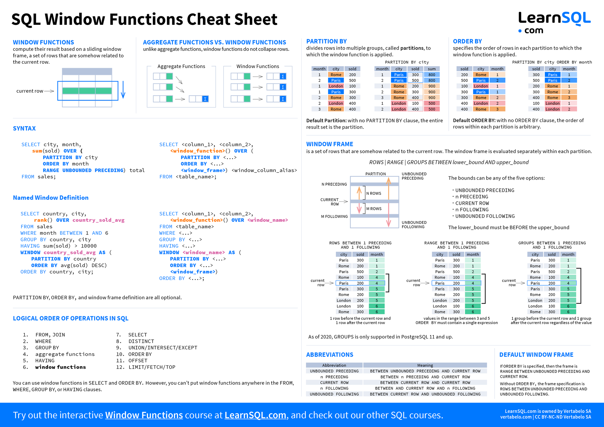
Window functions are one of the most powerful features in modern SQL. Like aggregate functions, they perform calculations across a set of rows. However, they do not collapse the rows. Instead, they return a calculated value for each row, based on a "window" of related rows.

This is perfect for tasks like ranking, running totals, and comparing a row to its neighbors.

The core of a window function is the OVER() clause, which defines the window of rows. It has two main sub-clauses:

• PARTITION BY: Divides the rows into groups (partitions). The window function is applied independently to each partition. This is similar to GROUP BY but doesn't collapse rows.
• ORDER BY: Orders the rows within each partition. This is essential for functions that depend on order, like ranking or running totals.

Types of Window Functions

Let's watch a video that walks through the most common types.

Let's review these functions with some practical examples.

a) Running Totals (SUM)

This is a classic use case. For each sale, you want to see the cumulative sales total for that customer up to that point in time.

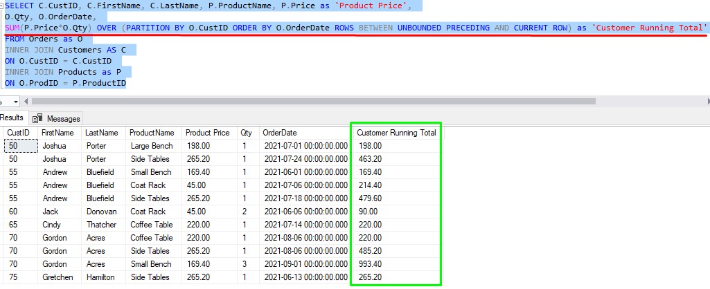
The key part of the query is:

SUM(sod.LineTotal) OVER (PARTITION BY soh.CustomerID ORDER BY soh.OrderDate) AS RunningTotal

• PARTITION BY soh.CustomerID: The running total restarts for each customer.
• ORDER BY soh.OrderDate: The sum accumulates in chronological order.

b) Ranking (RANK, DENSE_RANK, ROW_NUMBER)

Imagine you want to find the top 3 selling products within each product category.

WITH ProductSales AS (
    SELECT
        pc.Name AS Category,
        p.Name AS Product,
        SUM(sod.LineTotal) AS TotalSales
    FROM Sales.SalesOrderDetail AS sod
    JOIN Production.Product AS p ON sod.ProductID = p.ProductID
    JOIN Production.ProductSubcategory AS psc ON p.ProductSubcategoryID = psc.ProductSubcategoryID
    JOIN Production.ProductCategory AS pc ON psc.ProductCategoryID = pc.ProductCategoryID
    GROUP BY pc.Name, p.Name
)
SELECT
    Category,
    Product,
    TotalSales,
    DENSE_RANK() OVER (PARTITION BY Category ORDER BY TotalSales DESC) AS RankInCategory
FROM ProductSales
WHERE DENSE_RANK() OVER (PARTITION BY Category ORDER BY TotalSales DESC) <= 3;

• We use a Common Table Expression (CTE) ProductSales to first aggregate sales per product.
• DENSE_RANK() OVER (PARTITION BY Category ORDER BY TotalSales DESC): This ranks products within each Category based on their TotalSales in descending order. We use DENSE_RANK to avoid skipping ranks if there are ties.
• The final WHERE clause filters for the top 3 ranks in each category.

c) Year-over-Year Growth (LAG)

The LAG() function is perfect for comparing a row's value to a previous row's value. We can use it to calculate year-over-year (YoY) sales growth.

The logic for YoY growth is:
((CurrentMonthSales - SameMonthLastYearSales) / SameMonthLastYearSales) * 100

And LAG makes finding SameMonthLastYearSales straightforward:

LAG(MonthlyTotal, 12) OVER (ORDER BY SalesYear, SalesMonth)

This looks back 12 rows (months) in the ordered set to get the value from the previous year.

Conclusion

In this lesson, you've taken a significant step into writing powerful, data-centric queries directly in MSSQL. These skills are the bedrock of database optimization and complex feature development.

Here are the key takeaways:

• JOIN clauses (INNER, LEFT) are used to combine rows from multiple tables based on related columns.
• GROUP BY collapses many rows into a few summary rows, using aggregate functions like SUM() and COUNT() to compute values for each group.
• HAVING is used to filter the results of a GROUP BY based on the aggregated values.
• Window functions perform calculations across a set of related rows but, crucially, return a value for every single row without collapsing the result set. They are your tool for ranking, running totals, moving averages, and period-over-period comparisons.

Up Next:

You now have a solid grasp of what MSSQL can do with its native query language. In our next lesson, "Translate complex SQL queries into Laravel's Query Builder syntax," we will take the concepts you've learned here (JOINs, aggregations) and express them using Laravel's fluent, programmatic interface. This will bridge the gap between raw SQL power and clean, maintainable application code.