
Welcome back. In the previous lesson, you used conditional probability and Bayes’ rule to update a probability after observing evidence. We now turn from probabilities of events to numerical summaries of observed data: where values tend to lie, how widely they vary, and whether two measurements tend to move together.
By the end of this lesson, you will be able to calculate mean, variance, standard deviation, and covariance for a small dataset using NumPy—and, importantly, explain what each result does and does not mean. These summaries will become routine tools when profiling datasets during exploratory data analysis.
Center: the mean
Suppose four customers spent the following numbers of minutes in a support session:
The mean is the arithmetic average:
For this data:
The mean gives a central reference point. It does not have to be an observed value: no customer in this example spent exactly five minutes, but five is the balance point of the values.
In NumPy:
import numpy as np

minutes = np.array([2, 4, 6, 8])
mean_minutes = np.mean(minutes)

print(mean_minutes)  # 5.0
For a table-shaped array, the chosen axis determines what NumPy summarizes. If rows are observations and columns are variables, axis=0 calculates one mean per column:
data = np.array([
    [2, 9],
    [4, 7],
    [6, 5],
    [8, 3]
])

print(data.mean(axis=0))  # [5. 6.]
Here, the first column has mean ; the second has mean . NumPy collapses the rows and leaves one result per feature column.
Spread: variance and standard deviation
A mean alone can hide important differences. Consider these two sets:
Both have mean , but set is much more spread out. We need a measure of variability.
Variance
Variance measures the average squared distance from the mean. For a full population:
Return to the minutes example, , with mean .
| Value | Deviation | Squared deviation |
|---|---|---|
| 2 | 9 | |
| 4 | 1 | |
| 6 | 1 | |
| 8 | 9 |
The squared deviations sum to , so the population variance is:
Squaring is deliberate:
- Positive and negative deviations cannot cancel out.
- Larger deviations receive more weight.
- The result is always nonnegative.
The drawback is units: if the data are measured in minutes, variance is measured in minutes squared. That is mathematically useful but not always intuitive.
Standard deviation
The standard deviation returns variability to the original units by taking the square root of variance:
For the same observations:
A practical interpretation is: values typically sit on the order of minutes away from their mean, although this is not a promise that every individual value lies within that distance.
Read NumPy’s official var documentation to connect the variance formula to the axis and ddof arguments you will use in code.
In the opening description and Parameters section, read the function overview, then focus specifically on the explanations of axis and ddof. In the Notes section, read the denominator discussion. Notice that ddof=0 divides by N, while ddof=1 divides by N-1.
Population versus sample: why ddof matters
There are two common situations:
-
You have the complete population of interest.
For example, all four support sessions that occurred in a short pilot. Use the population convention:In NumPy, this is the default:
ddof=0. -
You have a sample intended to estimate a larger population.
For example, four support sessions sampled from all future sessions. Use the sample variance:In NumPy, use
ddof=1.
For the same four values, the sample variance is:
and the sample standard deviation is:
Using , often called Bessel’s correction, makes the sample variance a better estimator of population variance under the usual random-sampling assumptions. Do not mix conventions in the same comparison: if you use sample covariance, use sample standard deviations too.
Co-movement: covariance
Mean describes center; variance describes one variable’s spread. Covariance describes how two variables vary together.
Suppose we pair support-session minutes with the number of unresolved issues remaining afterward:
As session time rises, unresolved issues fall. The population covariance is:
The means are:
| Product | ||
|---|---|---|
The products sum to , so:
The sign supplies the main interpretation:
- Positive covariance: both variables tend to be above their means together, and below their means together.
- Negative covariance: when one tends to be above its mean, the other tends to be below its mean.
- Covariance near zero: no clear linear co-movement is visible in the data.
A zero covariance does not generally prove that two variables are independent. It only indicates that their linear co-movement cancels out. Nonlinear relationships can still exist.
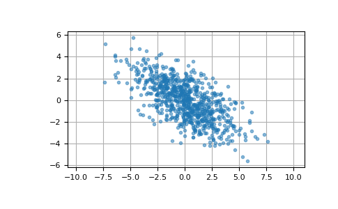
The artificial support-session example has a perfectly descending pattern. Real data are usually noisier, like the scatter plot, but the overall direction can still be negative.
Covariance magnitude is difficult to compare across datasets because it depends on measurement units. Changing minutes to seconds changes the covariance even when the underlying relationship is identical. A later lesson will use correlation to create a standardized comparison measure; for now, focus on covariance’s direction and its role in the covariance matrix.
Covariance matrices in NumPy
np.cov() returns a covariance matrix, not just one number. For two variables and , its structure is:
The diagonal contains variances. The off-diagonal entries contain covariances. The matrix is symmetric because:
One detail is especially important for tabular data: NumPy’s np.cov() assumes rows are variables by default. In machine-learning tables, we usually store rows as observations and columns as features, so use rowvar=False.
data = np.array([
    [2, 9],
    [4, 7],
    [6, 5],
    [8, 3]
])

sample_covariance = np.cov(data, rowvar=False)
population_covariance = np.cov(data, rowvar=False, bias=True)

print(sample_covariance)
print(population_covariance)
The first matrix uses the sample convention by default, dividing by :
[[ 6.66666667 -6.66666667]
 [-6.66666667  6.66666667]]
The second uses the population convention, dividing by :
[[ 5. -5.]
 [-5.  5.]]
Learn NumPy in 40 Minutes - Python NumPy Tutorial
Watch Tech With Tim’s “Learn NumPy in 40 Minutes” example to reinforce how statistical operations change when you choose an axis.
Watch the grade analysis. Treat each row as one observation and each column as one feature. Focus on why axis=0 produces one summary for each test column, while axis=1 produces one summary for each student row.
Concept-Level Micro-Challenge: summarize and verify a paired dataset
Type and run this 15-line NumPy program. It calculates both population and sample summaries, then verifies that the covariance matrix agrees with direct calculations.
import numpy as np
hours = np.array([2., 4., 6., 8.])
issues = np.array([9., 7., 5., 3.])
data = np.column_stack((hours, issues))
means = data.mean(axis=0)
pop_var = data.var(axis=0)
sample_std = data.std(axis=0, ddof=1)
sample_cov = np.cov(data, rowvar=False)
pop_cov = np.cov(data, rowvar=False, bias=True)
manual_cov = ((hours - hours.mean()) * (issues - issues.mean())).mean()
print("means:", means, "population variances:", pop_var)
print("sample standard deviations:", sample_std)
print("sample covariance matrix:\n", sample_cov)
assert np.isclose(pop_cov[0, 1], manual_cov)
assert np.allclose(pop_cov.diagonal(), pop_var)
You should observe:
- means of
[5., 6.]; - population variances of
[5., 5.]; - sample standard deviations near
[2.582, 2.582]; - a negative off-diagonal covariance;
- no assertion errors.
Read the two assertions carefully:
- The first confirms that the direct covariance formula equals the relevant off-diagonal matrix entry.
- The second confirms that covariance-matrix diagonals are the variances of the individual variables.
Before moving on, change the final issues value from 3. to 12. and run the code again. The covariance should become less negative or positive because the final observation now has high values for both features. This is a compact way to see that covariance depends on paired observations, not merely on each column’s separate distribution.
A compact interpretation checklist
When you see these statistics in an EDA notebook, ask:
| Statistic | Question it answers | Interpretation caution |
|---|---|---|
| Mean | Where is the numerical center? | Sensitive to extreme values. |
| Variance | How spread out are values, in squared units? | Magnitude depends on units. |
| Standard deviation | How much variation is present in original units? | Does not state a guaranteed range for individuals. |
| Covariance | Do two variables tend to move together or oppositely? | Magnitude depends on both variables’ units; it does not establish causation. |
For example, a negative covariance between support time and unresolved issues could support a useful investigation, but it cannot prove that longer sessions cause fewer unresolved issues. More complex cases may reflect issue severity, customer type, or how sessions are assigned.
Takeaways
You can summarize a numeric feature’s center and spread with:
Use NumPy’s mean, var, and std, choosing ddof=0 for a population description and ddof=1 when estimating population variance from a sample.
For paired measurements, covariance is:
Its sign indicates whether variables tend to move together or in opposite directions, while its raw magnitude remains dependent on measurement scale. In NumPy, np.cov(data, rowvar=False) is the appropriate starting point when rows are records and columns are features.
Next, you will put these summaries into visual form by creating correctly labelled univariate and bivariate plots with Matplotlib and Seaborn.
Can't find a good explanation? Sign up and we'll make it for you
Sign up