
Welcome back. In the previous lesson, you estimated partial derivatives and used the negative gradient to take a step downhill on a loss surface. That was about how to improve a model’s parameters. This lesson shifts to reasoning under uncertainty: how new evidence should change an estimate.
You will calculate conditional probabilities, distinguish the two directions of a conditional statement, and apply Bayes’ rule to a small diagnostic-test example. This is foundational for interpreting classification models later—especially when a rare outcome produces apparently convincing positive predictions.
Conditioning changes the reference group
Let and be events. The notation
is read as “the probability of , given .” Once you know that occurred, you no longer compare against the entire population. You restrict attention to the cases where is true.
Formally, provided ,
where means that both events occur.
For example, suppose 30 of 100 customers are subscribers, and 18 of those subscribers renew their plan. If means “renews” and means “is a subscriber,” then:
The denominator is 30—not 100—because the condition “is a subscriber” narrows the sample space to subscribers.
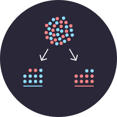
3.4 Probability Theory - Principles of Data Science | OpenStax
Read the OpenStax discussion to establish the “restricted sample space” interpretation of conditional probability, then see a diagnostic use of Bayes’ theorem.
In the subsection “Conditional Probability,” read the explanation beginning with the conditional-probability discussion. Then read Example 3.19 and focus on why the solution uses only the “23 and older” row as its denominator. In the “Bayes’ Theorem” subsection, read Example 3.21, especially the diagnostic example. Track carefully which probability is known before the test and which probability is being revised after observing a positive result.
Order matters
A frequent and consequential error is to reverse the direction of a conditional probability:
For a diagnostic test, define:
- : the person truly has the condition.
- : the test result is positive.
Then:
means “among people who have the condition, what fraction test positive?” This is the sensitivity or true-positive rate.
But the question a person normally asks after receiving a positive test is:
meaning “among people with positive test results, what fraction truly have the condition?” These are different questions because they use different denominators.
A test may be highly sensitive, yet a positive result may still have modest evidential value when the condition is rare or when false positives occur.
Bayes’ rule: reverse the conditional probability correctly
Bayes’ rule provides a disciplined way to go from to :
The overall probability of a positive result, , must include both ways a positive result can occur:
- the person has the condition and tests positive;
- the person does not have the condition but receives a false positive.
Thus,
Combining these gives the practical binary-diagnostic form:
The terms have useful names:
| Quantity | Meaning |
|---|---|
| Prior or base rate: prevalence before seeing the test | |
| Likelihood: sensitivity / true-positive rate | |
| False-positive rate | |
| Evidence: overall chance of a positive result | |
| Posterior: updated probability after a positive result |
A diagnostic example using both probabilities and counts
Consider a fictional screening process with these properties:
In words:
- The condition affects of the population.
- The test is positive for of people who have the condition.
- The test is falsely positive for of people without it.
First calculate the joint probability of having the condition and receiving a positive result:
Next, calculate the overall rate of positive tests:
Now Bayes’ rule gives:
So a positive result corresponds to about a probability that the condition is truly present—not .
A count-based view makes the denominator intuitive. Imagine exactly 10,000 screened people:
| Actual status | Positive test | Negative test | Total |
|---|---|---|---|
| Has condition | 180 | 20 | 200 |
| Does not have condition | 490 | 9,310 | 9,800 |
| Total | 670 | 9,330 | 10,000 |
Now the two conditional probabilities are visibly different:
The false positives matter because the condition is uncommon. There are many more people without the condition, so even a false-positive rate creates a substantial number of false alarms.
Bayes' Theorem Example: Drug Testing 🌿
Watch Steve Brunton’s “Bayes’ Theorem Example: Drug Testing” for a visual walkthrough of the same inverse-probability logic, including the role of prevalence and false positives.
Watch the first calculation. As the formula is assembled, identify the numerator as “true positives in the whole population” and the denominator as “all positive tests.” Focus on why a reasonably accurate test can still yield only a 50% posterior probability when the base rate is low.
In later classification lessons, this posterior has a familiar interpretation. If is the actual positive class and is a model’s positive prediction, then:
is the model’s precision (also called positive predictive value) for that population and decision threshold. Its value depends not only on the model’s ability to detect positive cases, but also on the outcome prevalence and false-positive rate.
Concept-Level Micro-Challenge: calculate a posterior with NumPy
Type and run this 15-line program. It calculates a conditional probability from the model assumptions, applies Bayes’ rule, and confirms the posterior using expected counts from a 10,000-person population.
import numpy as np
p_disease = 0.02
sensitivity = 0.90
false_positive_rate = 0.05
p_no_disease = 1 - p_disease
p_disease_and_positive = sensitivity * p_disease
p_positive = p_disease_and_positive + false_positive_rate * p_no_disease
p_disease_given_positive = p_disease_and_positive / p_positive
n = 10_000
true_positives = n * p_disease_and_positive
false_positives = n * false_positive_rate * p_no_disease
from_counts = true_positives / (true_positives + false_positives)
print(f"overall +: {p_positive:.3f}, posterior: {p_disease_given_positive:.3f}")
assert np.isclose(p_disease_and_positive / p_disease, sensitivity)
assert np.isclose(from_counts, p_disease_given_positive)
Expected output:
overall +: 0.067, posterior: 0.269
Read the checks as mathematical claims:
p_disease_and_positive / p_diseaserecovers , the sensitivity.from_countscalculates , which must agree with the Bayes posterior.- The code uses expected counts, not a random simulation, so it gives the exact proportions implied by the assumptions.
A useful parameter check: change p_disease from 0.02 to 0.20 while keeping test performance fixed. The posterior will rise sharply. This isolates the effect of the base rate: a positive result contains different information in different populations.
Common mistakes to catch now
-
Reversing the condition.
Sensitivity does not answer the post-test question . -
Using sensitivity as the final answer.
A sensitivity means the test detects of true cases. It does not mean that of positive results are true cases. -
Ignoring false positives.
The denominator must count positives from both actual cases and non-cases. -
Ignoring the base rate.
A rare event can produce a low posterior probability even after a positive test. -
Treating association as certainty.
A posterior probability updates uncertainty; it does not establish a causal explanation or a guaranteed individual outcome.
Takeaways
Conditional probability narrows the reference group:
The direction of conditioning matters:
Bayes’ rule reverses a conditional probability by combining the prior rate, likelihood, and total probability of the observed evidence:
For diagnostic and classification settings, a positive prediction must be interpreted in light of false positives and the base rate—not test sensitivity alone.
Next, you will calculate mean, variance, standard deviation, and covariance with NumPy, moving from probability rules to the numerical summaries used to describe real datasets.
Can't find a good explanation? Sign up and we'll make it for you
Sign up