Finite-Difference Gradients and Descent Directions

Welcome back. In the previous lesson, a dot product turned feature values and weights into a single score. Here, we use that same operation in a new role: it explains why the gradient tells us which small parameter change will increase or decrease a function most quickly.

You will treat a two-variable function as a local landscape, estimate its slopes numerically without differentiating it symbolically, combine those estimates into a gradient vector, and choose a step that lowers the function. This is the core calculation behind gradient descent, which you will implement more fully later in Month 1.

---

Partial derivatives: change one coordinate, hold the other fixed

Suppose a function depends on two inputs:

$$f(x,y)$$

At a particular point $(x_0,y_0)$, the partial derivative with respect to $x$ asks:

If $x$ changes slightly while $y$ stays fixed, how quickly does $f$ change?

Likewise, the partial derivative with respect to $y$ changes only $y$, holding $x$ fixed.

$$\frac{\partial f}{\partial x}(x_0,y_0)\text{and}\frac{\partial f}{\partial y}(x_0,y_0)$$

For a loss function in machine learning, you can interpret $x$ and $y$ as two model parameters. Each partial derivative measures how sensitive the loss is to one parameter, assuming the other is temporarily unchanged.

For example, let

$$f(x,y)=(x-3{)}^2+2(y+1{)}^2$$

and evaluate it at:

$$p=\left[\begin{array}{c}0\\ 2\end{array}\right]$$

The function value there is:

$$f(0,2)=(0-3{)}^2+2(2+1{)}^2=9+18=27$$

Rather than using calculus to obtain an exact derivative, we will estimate each slope by probing nearby points.

---

Finite differences: estimate a slope from nearby function values

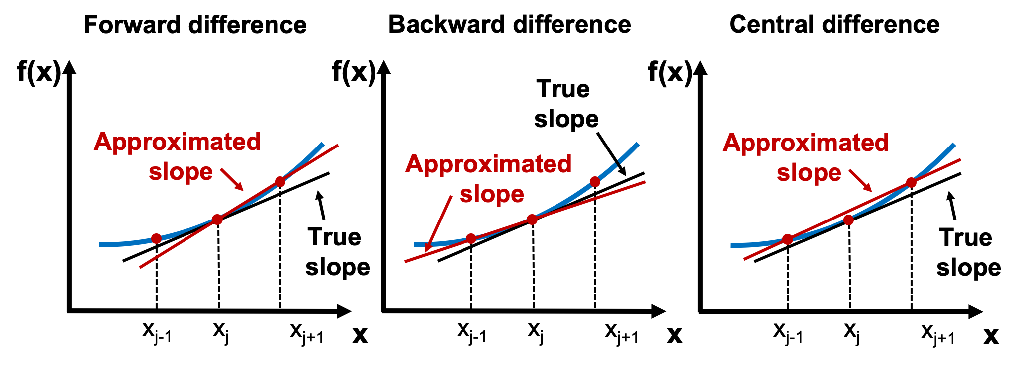
A finite difference replaces an infinitesimal change with a small, concrete step $h$. In one dimension, it approximates a tangent slope by a secant slope.

For the partial derivative with respect to $x$, keep $y$ constant and move only in the $x$ direction.

Forward difference

$$\frac{\partial f}{\partial x}(x_0,y_0)\approx \frac{f(x_0+h,y_0)-f(x_0,y_0)}{h}$$

This compares the current point with one point “forward” in the $x$ direction.

Backward difference

$$\frac{\partial f}{\partial x}(x_0,y_0)\approx \frac{f(x_0,y_0)-f(x_0-h,y_0)}{h}$$

This uses the point behind the current position.

Central difference

$$\frac{\partial f}{\partial x}(x_0,y_0)\approx \frac{f(x_0+h,y_0)-f(x_0-h,y_0)}{2h}$$

Central difference samples on both sides of the target point. For smooth functions, it is usually the preferred numerical estimate because its approximation error decreases more rapidly as $h$ becomes smaller.

The same pattern applies to $y$:

$$\frac{\partial f}{\partial y}(x_0,y_0)\approx \frac{f(x_0,y_0+h)-f(x_0,y_0-h)}{2h}$$

For a concise visual derivation of why central differences are typically more accurate than one-sided estimates, watch this segment.

A note on choosing $h$

Choosing $h$ involves a practical trade-off:

• If $h$ is too large, the secant line spans too much curvature and is a poor local approximation.
• If $h$ is extremely small, floating-point rounding can dominate the subtraction of nearly equal values.

For the small, well-scaled examples in this course, values such as 1e-4 or 1e-5 are sensible starting points. Numerical gradients are especially useful for checking an implementation; later, analytic gradients will usually be faster for actual model training.

---

Estimating two partial derivatives at one point

Return to:

$$f(x,y)=(x-3{)}^2+2(y+1{)}^2$$

at $(0,2)$. Let $h=0.001$.

To estimate the $x$-partial derivative, change $x$ while keeping $y=2$:

$$\frac{\partial f}{\partial x}(0,2)\approx \frac{f(0.001,2)-f(-0.001,2)}{2(0.001)}$$

The two function values are:

$$f(0.001,2)=27-6h+h^2$$ $$f(-0.001,2)=27+6h+h^2$$

Therefore:

$$\frac{f(h,2)-f(-h,2)}{2h}=\frac{-12h}{2h}=-6$$

So a small positive move in $x$ decreases $f$: the local $x$-slope is negative.

Now vary $y$ while keeping $x=0$:

$$\frac{\partial f}{\partial y}(0,2)\approx \frac{f(0,2+h)-f(0,2-h)}{2h}=12$$

Here, increasing $y$ increases $f$, so the $y$-slope is positive.

These two values are the components of the gradient.

---

Assemble the gradient and reverse it to descend

For a two-variable function, the gradient is:

$$\nabla f(x,y)=\left[\begin{array}{c}\frac{\partial f}{\partial x}(x,y)\\ \frac{\partial f}{\partial y}(x,y)\end{array}\right]$$

At $(0,2)$, our finite-difference estimates give:

$$\nabla f(0,2)\approx \left[\begin{array}{c}-6\\ 12\end{array}\right]$$

The gradient points in the local direction of steepest increase. Therefore, its negative points in the local direction of steepest decrease:

$$-\nabla f(0,2)=\left[\begin{array}{c}6\\ -12\end{array}\right]$$

This tells us to increase $x$ and decrease $y$.

The connection to the prior dot-product lesson is precise. For a small position change $\Delta p$,

$$f(p+\Delta p)\approx f(p)+\nabla f(p{)}^T\Delta p$$

If we choose:

$$\Delta p=-\eta \nabla f(p)$$

where $\eta >0$ is a small step size, then:

$$\nabla f(p{)}^T\Delta p=-\eta \nabla f(p{)}^T\nabla f(p)=-\eta \Vert \nabla f(p){\Vert }^2$$

This is negative whenever the gradient is nonzero. Thus, for a sufficiently small $\eta$, the function should decrease locally.

Using $\eta =0.1$:

$$p_{\text{new}}=\left[\begin{array}{c}0\\ 2\end{array}\right]-0.1\left[\begin{array}{c}-6\\ 12\end{array}\right]=\left[\begin{array}{c}0.6\\ 0.8\end{array}\right]$$

The loss falls from:

$$f(0,2)=27$$

to:

$$f(0.6,0.8)=12.24$$

The direction was right; the step successfully moved downhill.

A zero gradient is a special case: it means there is no first-order uphill or downhill direction at that exact point. It may be a minimum, a maximum, or a saddle point, so zero gradient alone does not prove that a function is minimized.

---

Numerical gradients in NumPy

The CS231n notes provide a general pattern for numerical gradients: alter one coordinate, evaluate the function, restore the original coordinate, then repeat for each coordinate.

In practice, use .copy() when making perturbed versions of a parameter vector. This avoids accidentally changing the original evaluation point and corrupting later estimates.

---

Concept-Level Micro-Challenge: central-difference gradient and one descent step

Type and run this 15-line NumPy program. It estimates both partial derivatives using central differences, then takes one negative-gradient step.

import numpy as np
def loss(p):
    x, y = p
    return (x - 3)**2 + 2 * (y + 1)**2
p = np.array([0.0, 2.0]); h = 1e-4
grad = np.zeros_like(p)
for j in range(p.size):
    plus = p.copy()
    minus = p.copy()
    plus[j] += h; minus[j] -= h
    grad[j] = (loss(plus) - loss(minus)) / (2 * h)
p_new = p - 0.1 * grad
print("gradient:", grad, "old/new loss:", loss(p), loss(p_new))
assert np.allclose(grad, [-6.0, 12.0], atol=1e-6)
assert loss(p_new) < loss(p)

Your expected gradient is approximately:

$$[-6,12]$$

Read the loop carefully:

• At j = 0, only the first coordinate changes, so the code estimates $\partial f/\partial x$.
• At j = 1, only the second coordinate changes, so it estimates $\partial f/\partial y$.
• p - 0.1 * grad moves in the negative-gradient direction.

As a brief self-check, change the final update to p + 0.1 * grad. The assertion that the loss decreases should fail, because this update deliberately moves uphill.

---

Common mistakes to catch early

1. Changing both variables for one partial derivative.
   To estimate $\partial f/\partial x$, alter only p[0]; keep p[1] fixed. Changing both coordinates estimates movement along a diagonal, not a partial derivative.

2. Forgetting the denominator $2h$ in central difference.
   The two samples are $2h$ apart, not $h$ apart.

3. Using the gradient as a descent direction.
   The gradient points uphill. Use -grad or subtract learning_rate * grad.

4. Taking a step that is too large.
   A gradient is local information. A direction can be correct while an oversized step overshoots into a higher-loss region.

5. Mutating the base point accidentally.
   Use plus = p.copy() and minus = p.copy(). If the base point changes inside the loop, the partial derivatives no longer refer to the same location.

---

Takeaways

A partial derivative measures local change along one coordinate while all other coordinates remain fixed. Finite differences approximate that derivative using nearby function values; central difference is usually the strongest default:

$$\frac{\partial f}{\partial x}(x,y)\approx \frac{f(x+h,y)-f(x-h,y)}{2h}$$

For a two-variable function, assemble both estimates into the gradient:

$$\nabla f(x,y)=\left[\begin{array}{c}\partial f/\partial x\\ \partial f/\partial y\end{array}\right]$$

The gradient points toward local steepest increase. Its negative gives a local descent direction, and a small update of the form

$$p_{\text{new}}=p-\eta \nabla f(p)$$

should reduce the function when the step size is appropriate.

Next, you will switch from optimization math to probability, calculating conditional probabilities and applying Bayes’ rule in a compact diagnostic example.