Computing and Interpreting Vector Dot Products in NumPy

Welcome back. You have already separated element-wise multiplication from matrix multiplication: * keeps one result per entry, while @ combines rows and columns. A vector dot product is the smallest useful case of that combination: it turns two equal-length vectors into one number.

In this lesson, you will compute dot products with NumPy and interpret them in two complementary ways:

• as a weighted sum, the calculation underlying linear-model scores; and
• as an indicator of directional alignment, which can support a similarity comparison when vector magnitudes are handled appropriately.

Plan for about 35–40 minutes, including a compact NumPy micro-challenge.

---

From paired products to one scalar

For two vectors of the same length,

$$x=\left[\begin{array}{c}{x}_1\\ x_2\\ ⋮\\ x_n\end{array}\right]w=\left[\begin{array}{c}{w}_1\\ w_2\\ ⋮\\ w_n\end{array}\right]$$

their dot product is:

$$x\cdot w=x_1{w}_1+x_2{w}_2+\cdots +x_n{w}_n=\sum _{j=1}^n{x}_j{w}_j$$

The process has two stages:

1. Multiply corresponding entries.
2. Sum the resulting products.

For example:

$$x=\left[\begin{array}{c}2\\ -1\\ 0.5\end{array}\right]w=\left[\begin{array}{c}0.8\\ -0.4\\ 2.0\end{array}\right]$$

First compute the per-feature contributions:

$$x\ast w=\left[\begin{array}{c}2(0.8)\\ -1(-0.4)\\ 0.5(2.0)\end{array}\right]=\left[\begin{array}{c}1.6\\ 0.4\\ 1.0\end{array}\right]$$

Then add them:

$$x\cdot w=1.6+0.4+1.0=3.0$$

This comparison should now feel familiar:

import numpy as np

x = np.array([2.0, -1.0, 0.5])
w = np.array([0.8, -0.4, 2.0])

contributions = x * w     # one contribution per feature
score = x @ w             # one scalar: sum of contributions

Here, contributions is [1.6, 0.4, 1.0], while score is 3.0.

For two one-dimensional NumPy arrays, these forms compute the same dot product:

np.dot(x, w)
x @ w

Both require the vectors to have equal length. The output is a scalar, not a vector:

print((x @ w).shape)  # ()

The empty shape () is NumPy’s way of saying “zero-dimensional scalar result.”

To reinforce the computational mechanics, watch this short portion of The Dot Product — Topic 14 of Machine Learning Foundations by Jon Krohn.

---

Interpretation 1: a weighted sum of features

The most immediately useful machine-learning interpretation is that a dot product is a weighted sum.

Suppose a record has three numeric features. A model assigns one coefficient, or weight, to each feature:

Quantity	Meaning	Value
$x_1$	first feature value	$2.0$
$x_2$	second feature value	$-1.0$
$x_3$	third feature value	$0.5$
$w_1$	weight for feature 1	$0.8$
$w_2$	weight for feature 2	$-0.4$
$w_3$	weight for feature 3	$2.0$

The resulting score is:

$$s=x\cdot w=3.0$$

Each product $x_j{w}_j$ is that feature’s contribution to the total score:

• A feature with a positive value and positive weight raises the score.
• A feature with a positive value and negative weight lowers the score.
• A negative feature value reverses the contribution’s sign.
• A weight of zero means the feature contributes nothing to this linear score.

This is why inspecting only a model weight can be misleading. The impact for one observation depends on both the feature value and its weight.

Most tabular ML data consists of many observations, each with the same set of features. Put those observations into a feature matrix $X$, where rows are records and columns are features:

$$X=\left[\begin{array}{ccc}2.0& -1.0& 0.5\\ 0.0& 3.0& 1.0\end{array}\right]w=\left[\begin{array}{c}0.8\\ -0.4\\ 2.0\end{array}\right]$$

Then:

$$Xw=\left[\begin{array}{c}3.0\\ 0.8\end{array}\right]$$

In NumPy:

X = np.array([
    [2.0, -1.0, 0.5],
    [0.0, 3.0, 1.0]
])

w = np.array([0.8, -0.4, 2.0])

scores = X @ w
print(scores)  # [3.  0.8]

This is matrix multiplication, but each output value is specifically a row-vector dot product:

$$(X@w{)}_i=X_{i,:}\cdot w$$

So X @ w produces one weighted score per row. This operation will reappear when you implement linear regression and logistic regression from scratch.

A model often also includes an intercept, or bias:

$$s=x\cdot w+b$$

The dot product aggregates feature contributions; the bias shifts every score by the same baseline amount. For now, keep those roles separate.

---

Interpretation 2: directional alignment and similarity

A dot product also has a geometric interpretation:

$$x\cdot y=\Vert x\Vert \Vert y\Vert \cos (\theta )$$

where $\theta$ is the angle between the vectors.

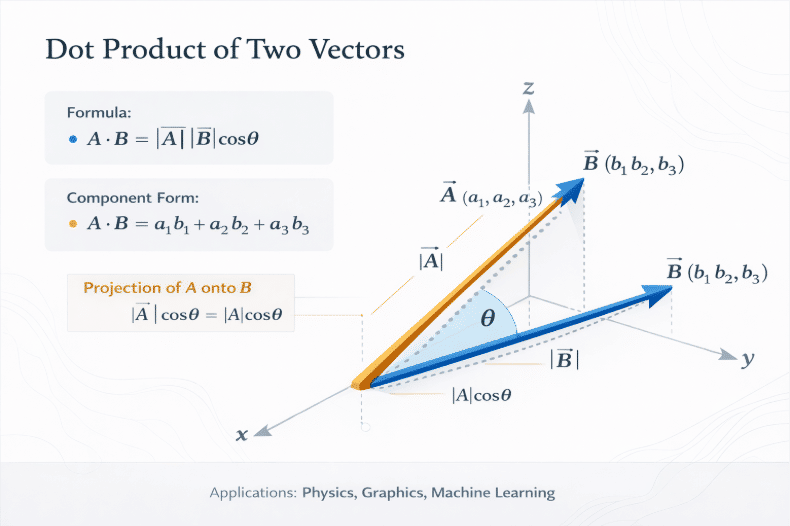
This formula gives a useful sign-based interpretation:

• If $x\cdot y>0$, the vectors point generally in similar directions.
• If $x\cdot y=0$, they are perpendicular, or orthogonal.
• If $x\cdot y<0$, they point generally in opposing directions.

For example:

$$a=\left[\begin{array}{c}1\\ 0\end{array}\right]b=\left[\begin{array}{c}0\\ 1\end{array}\right]c=\left[\begin{array}{c}-2\\ 0\end{array}\right]$$

Then:

$$a\cdot b=0$$

because the vectors are perpendicular, while:

$$a\cdot c=-2$$

because they point in opposite directions.

a = np.array([1.0, 0.0])
b = np.array([0.0, 1.0])
c = np.array([-2.0, 0.0])

print(a @ b)  # 0.0
print(a @ c)  # -2.0

An important caveat about “similarity”

A raw dot product is affected by both direction and magnitude. A long vector can receive a large dot product even if its direction is not the closest match.

When “similarity” should mean directional similarity independent of scale, use cosine similarity:

$$\text{cosine similarity}(x,y)=\frac{x\cdot y}{\Vert x\Vert \Vert y\Vert }$$

For nonzero vectors, cosine similarity ranges from $-1$ to $1$:

• $1$: exactly the same direction;
• $0$: perpendicular directions;
• $-1$: exactly opposite directions.

In NumPy, the calculation is:

cosine_similarity = (x @ y) / (np.linalg.norm(x) * np.linalg.norm(y))

This formula is valid only when neither vector has norm zero. Later, when working with real data, you will need to guard against all-zero vectors before dividing.

The practical distinction is:

• Use a raw dot product when magnitude is meaningful, such as a weighted model score.
• Use cosine similarity when you want to compare directions or patterns while ignoring overall scale.

---

Concept-Level Micro-Challenge: inspect contributions and batch scores

Type and run this 15-line NumPy program. Before executing it, calculate the first score by hand and predict the shape of batch_scores.

import numpy as np
x = np.array([2.0, -1.0, 0.5])
w = np.array([0.8, -0.4, 2.0])
contributions = x * w
score = np.dot(x, w)
manual_score = contributions.sum()
X = np.array([[2.0, -1.0, 0.5], [0.0, 3.0, 1.0]])
batch_scores = X @ w
print("contributions:", contributions)
print("single score:", score)
print("batch scores:", batch_scores)
assert contributions.shape == (3,)
assert np.isclose(score, 3.0)
assert np.isclose(score, manual_score)
assert batch_scores.shape == (2,)
assert np.allclose(batch_scores, [3.0, 0.8])

Interpret your result rather than treating the assertions as the endpoint:

• The three values in contributions are individual feature contributions.
• score is their sum: one weighted score for one record.
• batch_scores contains one dot product per row of X.

If you change only the second weight from -0.4 to 0.4, identify which contributions change sign and explain why. This is a compact way to test whether you can reason from the formula rather than only call NumPy functions.

---

A debugging checklist for dot products

When a dot-product calculation fails or produces a surprising value, check these points in order:

1. Confirm the intended operation.
   Use x * w to retain per-feature products; use x @ w or np.dot(x, w) to sum those products into a scalar.

2. Inspect shapes.

   print(x.shape, w.shape)
   

   For vector dot products, both should normally have shape (n,).

3. Check a contribution vector.

   print(x * w)
   

   A negative contribution is not automatically an error. It may reflect a negative feature, a negative weight, or both.

4. Calculate one result manually.
   For a short vector, manually add the products. For a matrix $X$, manually verify one row score.

5. Keep feature order fixed.
   The first value in x must correspond to the first weight in w, and so on. Equal lengths alone do not guarantee meaningful alignment.

That final point becomes critical once data is stored in DataFrames: a model weight vector is meaningful only when its feature ordering matches the preprocessing output.

---

Takeaways

A vector dot product multiplies corresponding entries and sums them into a single scalar:

$$x\cdot w=\sum _{j=1}^n{x}_j{w}_j$$

In NumPy, use np.dot(x, w) or x @ w for equal-length one-dimensional arrays.

You can interpret the result in two ways:

• As a weighted sum, where each term $x_j{w}_j$ is one feature’s contribution to a model score.
• As a measure of alignment, with positive, zero, and negative results indicating broadly aligned, perpendicular, and opposing directions. For scale-independent directional comparison, normalize to cosine similarity.

For a feature matrix, X @ w computes one weighted dot-product score per row. Next, you will move from these linear combinations to partial derivatives and gradients, which tell us how to change model parameters so that an error function decreases.