Computing and Interpreting Descriptive Statistics

Welcome back. In the previous lesson, you used the chain rule to track how a small change propagates through a computation. We now shift from functions to datasets: instead of asking how an output changes, we ask what a collection of measurements looks like.

For speech work, these summaries are practical diagnostics. You may inspect average utterance duration, variation in loudness, or whether duration and transcript length tend to move together. By the end of this lesson, you will be able to compute and interpret a dataset’s mean, variance, and covariance, while being explicit about whether the observed data is a complete population or a sample.

---

Center: the mean

Suppose a small speech-data audit contains the following paired measurements:

Clip	Duration $d$ (seconds)	Transcript tokens $w$
1	1	2
2	2	3
3	3	4
4	4	7

Each row describes one paired observation: the duration and token count belong to the same clip. This pairing will matter when we reach covariance.

For one variable $x$, the mean is its total divided by the number of observations $n$:

$$\bar{x}=\frac{1}{n}\sum _{i=1}^n{x}_i.$$

The bar in $\bar{x}$ means “sample mean,” the mean calculated from observed values. If we truly have every member of a population, we commonly write its mean as $\mu$. The calculation is structurally identical; the notation tells us what the data represent.

For the durations,

$$\bar{d}=\frac{1+2+3+4}{4}=2.5\text{ seconds}.$$

For the token counts,

$$\bar{w}=\frac{2+3+4+7}{4}=4\text{ tokens}.$$

The mean is a center of balance, not necessarily a value that appeared in the data. No clip is $2.5$ seconds long, but $2.5$ seconds is still the central reference value for this set of durations.

For a feature vector with several measurements per example, compute one mean per column. If each observation is

$${\mathbf{x}}_i=\left[\begin{array}{c}{d}_i\\ w_i\end{array}\right],$$

then the mean vector is

$$\bar{\mathbf{x}}=\frac{1}{n}\sum _{i=1}^n{\mathbf{x}}_i=\left[\begin{array}{c}\bar{d}\\ \bar{w}\end{array}\right]=\left[\begin{array}{c}2.5\\ 4\end{array}\right].$$

A mean vector is useful because real speech datasets have many numerical columns: duration, RMS energy, number of tokens, speaking rate, and so on.

---

Spread: variance and standard deviation

The mean alone hides an important distinction. These two duration datasets have the same mean:

$$A=[2,2,2,2],$$ $$B=[0.5,1.5,2.5,3.5].$$

Both have mean $2$ seconds. Yet Dataset A contains clips of identical duration, while Dataset B has a substantial spread. Variance measures that spread around the mean.

First calculate each deviation from the mean:

$$x_i-\bar{x}.$$

If we merely summed deviations, positive and negative values would always cancel:

$$\sum _{i=1}^n(x_i-\bar{x})=0.$$

Variance avoids cancellation by squaring every deviation before averaging.

If your dataset is the full population of interest, use the population variance:

$${\sigma }^2=\frac{1}{n}\sum _{i=1}^n(x_i-\mu {)}^2.$$

If the data is a sample used to estimate variation in a larger population, use the sample variance:

$$s^2=\frac{1}{n-1}\sum _{i=1}^n(x_i-\bar{x}{)}^2.$$

For most empirical datasets in ML, the word “sample” is statistically appropriate: a training corpus is usually only a subset of all possible future speakers, recording environments, and utterances. The $n-1$ denominator compensates for the fact that the sample mean was estimated from the same observations, which otherwise makes the observed deviations systematically too small for estimating population variability.

Worked variance calculation

Return to the four clip durations. Their mean is $2.5$ seconds.

$d_i$	$d_i-\bar{d}$	$(d_i-\bar{d}{)}^2$
1	$-1.5$	$2.25$
2	$-0.5$	$0.25$
3	$0.5$	$0.25$
4	$1.5$	$2.25$
Total	$0$	$5$

If these four clips are treated as the entire dataset of interest, their variance is

$${\sigma }_d^2=\frac{5}{4}=1.25{\text{ seconds}}^2.$$

If they are a sample from a larger speech population, the sample variance is

$$s_d^2=\frac{5}{3}\approx 1.67{\text{ seconds}}^2.$$

Variance has squared units. Duration variance is measured in seconds squared, which is mathematically meaningful but less intuitive in conversation. The standard deviation restores the original units by taking the square root:

$$s_d=\sqrt{s_d^2}.$$

For the sample calculation,

$$s_d=\sqrt{1.67}\approx 1.29\text{ seconds}.$$

Interpretation: the durations typically differ from their mean of $2.5$ seconds by a scale of roughly $1.29$ seconds. This is not a promise that every clip lies within one standard deviation; it is a summary of overall dispersion.

What variance tells you in speech data

A large variance can be expected or problematic depending on what is being measured:

• Duration: high variance may be normal in natural conversational data, but might reveal inconsistent segmentation in a dataset intended for short commands.
• Audio level: unusually high variance can indicate inconsistent gain normalization across sources.
• Transcript length: high variation affects batching efficiency and model memory use.
• Feature values: features with very different variances can cause optimization issues, which is one reason feature normalization is common in ML.

Variance is always nonnegative:

$$s^2\ge 0.$$

A variance of zero means every observed value is identical. It does not mean that the variable is “good,” merely that it does not vary in the data.

---

Co-movement: covariance

Variance asks: How much does one variable vary around its own mean?

Covariance asks: How do two variables vary together around their respective means?

The sample covariance of variables $x$ and $y$ is

$$s_{xy}=\frac{1}{n-1}\sum _{i=1}^n(x_i-\bar{x})(y_i-\bar{y}).$$

The population version uses ${\mu }_x$, ${\mu }_y$, and denominator $n$:

$${\sigma }_{xy}=\frac{1}{n}\sum _{i=1}^n(x_i-{\mu }_x)(y_i-{\mu }_y).$$

The core operation is a product of two centered deviations. Its sign carries the intuition:

Position relative to the means	Deviation product	Contribution
Both values above their means	positive times positive	Positive
Both values below their means	negative times negative	Positive
One above, one below	positive times negative	Negative

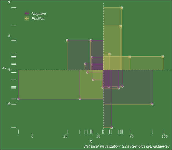
Covariance therefore summarizes whether deviations tend to have the same sign or opposing signs.

Worked covariance calculation

For the speech-clip dataset,

$$\bar{d}=2.5,$$ $$\bar{w}=4.$$

Now calculate the paired deviations and their products.

Clip	$d_i-\bar{d}$	$w_i-\bar{w}$	Product
1	$-1.5$	$-2$	$3$
2	$-0.5$	$-1$	$0.5$
3	$0.5$	$0$	$0$
4	$1.5$	$3$	$4.5$
Total			$8$

Using the sample convention,

$$s_{dw}=\frac{8}{4-1}=\frac{8}{3}\approx 2.67\text{ seconds}\cdot \text{tokens}.$$

The covariance is positive. In this small dataset, clips longer than the average tend also to have more tokens than the average; clips shorter than average tend to have fewer. That is consistent with a positive linear association between duration and transcript length.

The units are the product of both variables’ units:

$$\text{seconds}\cdot \text{tokens}.$$

That unusual unit is a clue that raw covariance magnitude is difficult to compare across differently scaled variables. If durations were converted from seconds to milliseconds, the numerical covariance would become $1000$ times larger even though the underlying relationship had not changed. Later, correlation will standardize covariance to make a unit-free relationship measure.

Three careful interpretations

Use covariance cautiously:

1. Positive covariance means the variables tend to move together relative to their means. It does not prove that one causes the other.
2. Negative covariance means one tends to be above its mean when the other is below its mean.
3. Zero covariance means no linear co-movement on average. It does not prove the variables are independent; a nonlinear relationship can still be present.

For example, if an acoustic feature rises for very soft and very loud speech but falls in the middle, the overall linear covariance with loudness could be near zero despite a meaningful curved relationship.

---

Variance as a special covariance

Variance is covariance of a variable with itself:

$$s_{xx}=\frac{1}{n-1}\sum _{i=1}^n(x_i-\bar{x})(x_i-\bar{x}).$$

Since multiplying a quantity by itself squares it,

$$s_{xx}=\frac{1}{n-1}\sum _{i=1}^n(x_i-\bar{x}{)}^2=s_x^2.$$

This connection lets us collect a dataset’s variances and covariances into a covariance matrix. For duration and token count:

$$S=\left[\begin{array}{cc}{s}_d^2& s_{dw}\\ s_{wd}& s_w^2\end{array}\right].$$

From our four clips,

$$S=\left[\begin{array}{cc}5/3& 8/3\\ 8/3& 14/3\end{array}\right].$$

Read the matrix as follows:

• The diagonal contains variances.
• The off-diagonal entries contain covariances.
• It is symmetric because $s_{dw}=s_{wd}$.

This is an important bridge to ML notation. If a data matrix $X$ has shape $n\times p$, with rows as examples and columns as numeric features, let $X_c$ be the centered matrix formed by subtracting each column mean. The sample covariance matrix is

$$S=\frac{1}{n-1}{X}_c^{\mathsf{T}}{X}_c.$$

The shape check is useful:

$$X_c^{\mathsf{T}}{X}_c\text{ has shape }(p\times n)(n\times p)=p\times p.$$

Each entry combines deviations for one feature with deviations for another. This is exactly why the diagonal entries are variances and the off-diagonal entries are covariances.

---

Computing reliably in NumPy

Hand calculation is essential for understanding the definitions. In practice, use library functions, but state the convention rather than silently accepting defaults.

import numpy as np

# Rows are clips; columns are [duration_seconds, token_count].
features = np.array([
    [1.0, 2.0],
    [2.0, 3.0],
    [3.0, 4.0],
    [4.0, 7.0],
])

means = features.mean(axis=0)

# Population-style summaries: divide by n.
population_variances = features.var(axis=0, ddof=0)
population_covariance = np.cov(features, rowvar=False, ddof=0)

# Sample-style summaries: divide by n - 1.
sample_variances = features.var(axis=0, ddof=1)
sample_covariance = np.cov(features, rowvar=False, ddof=1)

print(means)
print(sample_variances)
print(sample_covariance)

The expected sample results are approximately:

means
# [2.5, 4.0]

sample_variances
# [1.66666667, 4.66666667]

sample_covariance
# [[1.66666667, 2.66666667],
#  [2.66666667, 4.66666667]]

A few implementation checks prevent common errors:

• Use axis=0 when each column is a feature and each row is an observation.
• Ensure covariance columns are aligned by row. Pairing a clip’s duration with another clip’s transcript length makes the statistic meaningless.
• Set ddof deliberately. In NumPy, ddof=0 uses $n$; ddof=1 uses $n-1$.
• Confirm the covariance matrix is symmetric, allowing for tiny floating-point differences.
• Do not compare raw covariance magnitudes across variables with different scales without considering their units.

---

Key takeaways

• The mean is the central average:

$$\bar{x}=\frac{1}{n}\sum _{i=1}^n{x}_i.$$

• Variance is the average squared deviation from the mean. It measures spread and is never negative.
• Use denominator $n$ for a complete population and $n-1$ when estimating population variability from a sample.
• Standard deviation is the square root of variance and returns to the original units.
• Covariance averages the product of paired deviations:

$$s_{xy}=\frac{1}{n-1}\sum _{i=1}^n(x_i-\bar{x})(y_i-\bar{y}).$$

• Positive covariance indicates joint upward or downward deviations; negative covariance indicates opposite deviations. Its raw magnitude depends on scale.
• A covariance matrix places variances on its diagonal and covariances off the diagonal.

Next, you will use probability to reason about uncertainty in a classification setting, then apply conditional probability and Bayes’ rule.