Conditional Probability and Bayes’ Rule for Classification

Good to see you again. In the previous lesson, you summarized numerical speech-data properties with means, variances, and covariances. Those are descriptive tools: they tell you what a dataset looks like. This lesson moves to uncertainty about an individual example: given some evidence, how should a classifier’s belief change?

Conditional probability and Bayes’ rule are especially important whenever an apparently convincing signal is rare in real traffic. A speech-activity detector may flag audio as containing speech; a quality-control system may flag a clipped recording; a wake-word detector may trigger. The operational question is often not “how often does the detector fire when the condition is present?” but rather “when it fires, how likely is the condition actually present?”

By the end, you will be able to distinguish those questions, calculate conditional probabilities, and use Bayes’ rule to obtain a posterior class probability.

---

Conditional probability: restrict the population first

Let $A$ and $B$ be events. The notation

$$P(A\mid B)$$

is read as “the probability of $A$, given $B$.” The vertical bar means that we already know $B$ occurred.

The key move is to restrict the population to cases where $B$ is true. Among that reduced population, ask what fraction also belongs to $A$.

Formally, provided that $P(B)>0$,

$$P(A\mid B)=\frac{P(A\cap B)}{P(B)}.$$

Here, $A\cap B$ means that both events occur.

Suppose a batch contains $100$ audio clips:

• $30$ contain speech.
• $20$ are recorded on a mobile device.
• $12$ both contain speech and were recorded on a mobile device.

The unconditional probability that a randomly selected clip contains speech is

$$P(\text{speech})=\frac{30}{100}=\mathrm{0.30.}$$

But if you already know that the clip was recorded on a mobile device, the relevant population has only $20$ clips. Of those, $12$ contain speech:

$$P(\text{speech}\mid \text{mobile})=\frac{12}{20}=\mathrm{0.60.}$$

The condition changes the denominator. It does not merely add another fact to a sentence.

Conditional probabilities are directional

A common and consequential error is to reverse the condition:

$$P(A\mid B)\ne P(B\mid A)$$

in general.

For the audio example,

$$P(\text{speech}\mid \text{mobile})=\frac{12}{20}=0.60,$$

but

$$P(\text{mobile}\mid \text{speech})=\frac{12}{30}=\mathrm{0.40.}$$

Both calculations use the same overlap of $12$ clips, but they answer different questions and use different denominators.

This distinction becomes central in classification:

Quantity	What it asks
$P(\text{flag}\mid \text{condition})$	If the true condition exists, how often does the system flag it?
$P(\text{condition}\mid \text{flag})$	If the system flags it, how likely is the true condition?

The first is a property of the system’s behavior on a known class. The second is the probability an operator or downstream system usually needs after observing the flag.

---

Bayes’ rule: reversing a conditional probability

Bayes’ rule relates these two directions. Start with the joint probability that both $A$ and $B$ occur:

$$P(A\cap B)=P(A\mid B)P(B).$$

We can write the same joint probability in the other direction:

$$P(A\cap B)=P(B\mid A)P(A).$$

Since both expressions describe the same joint event,

$$P(A\mid B)P(B)=P(B\mid A)P(A).$$

Dividing by $P(B)$ gives Bayes’ rule:

$$P(A\mid B)=\frac{P(B\mid A)P(A)}{P(B)}.$$

The terms have useful names:

$$\underset{\text{posterior}}{\underbrace{P(A\mid B)}}=\frac{\underset{\text{likelihood}}{\underbrace{P(B\mid A)}}\underset{\text{prior}}{\underbrace{P(A)}}}{\underset{\text{evidence}}{\underbrace{P(B)}}}.$$

• The prior is the probability of the class before observing the evidence.
• The likelihood describes how compatible the observed evidence is with that class.
• The posterior is the updated probability after observing the evidence.
• The evidence normalizes the result so that the posterior is a valid probability.

For a two-class problem, where $A$ and $\bar{A}$ are mutually exclusive and cover all possibilities, the evidence is found with the law of total probability:

$$P(B)=P(B\mid A)P(A)+P(B\mid \bar{A})P(\bar{A}).$$

Substituting this into Bayes’ rule produces the version most useful for a binary classification calculation:

$$P(A\mid B)=\frac{P(B\mid A)P(A)}{P(B\mid A)P(A)+P(B\mid \bar{A})P(\bar{A})}.$$

---

A classification calculation with natural counts

Consider a hypothetical speech-activity flagger operating on short windows from an always-on audio stream. Let:

• $S$: the window truly contains speech.
• $F$: the system flags the window as speech.

Suppose the deployment environment has these properties:

$$P(S)=0.02,$$

so only $2\%$ of windows actually contain speech.

The system detects $90\%$ of true speech windows:

$$P(F\mid S)=\mathrm{0.90.}$$

But it also incorrectly flags $10\%$ of non-speech windows:

$$P(F\mid \bar{S})=\mathrm{0.10.}$$

The question after the system fires is:

$$P(S\mid F)=?$$

It is tempting to answer $90\%$, but $90\%$ is $P(F\mid S)$, not $P(S\mid F)$. It tells us about the flagger’s response to known speech, not about the composition of all flagged windows.

Natural counts make the calculation concrete. Imagine $10,000$ incoming audio windows.

• Since speech occurs in $2\%$ of windows, $200$ windows contain speech.
• The other $9,800$ windows contain no speech.
• The flagger catches $90\%$ of the $200$ true-speech windows, producing $180$ true positives.
• It incorrectly flags $10\%$ of the $9,800$ non-speech windows, producing $980$ false positives.

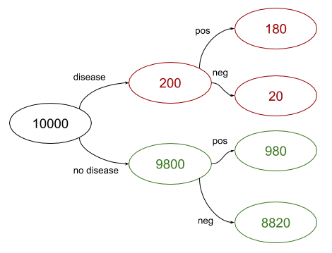
Among all flagged windows, there are

$$180+980=1160$$

flags. Only $180$ correspond to actual speech. Therefore,

$$P(S\mid F)=\frac{180}{1160}\approx \mathrm{0.155.}$$

So the posterior probability is about $15.5\%$:

$$P(S\mid F)\approx 15.5\%.$$

The same result follows directly from Bayes’ rule:

$$P(S\mid F)=\frac{P(F\mid S)P(S)}{P(F\mid S)P(S)+P(F\mid \bar{S})P(\bar{S})}.$$

Substitute the given probabilities:

$$P(S\mid F)=\frac{0.90\cdot 0.02}{(0.90\cdot 0.02)+(0.10\cdot 0.98)}.$$ $$P(S\mid F)=\frac{0.018}{0.116}\approx \mathrm{0.155.}$$

The low posterior does not mean the flagger has no value. Before the flag, the chance of speech was only $2\%$. After a flag, it is about $15.5\%$, a substantial update. But it may still be too uncertain to trigger an expensive downstream ASR model without additional filtering or a higher decision threshold.

---

The base-rate effect in speech systems

Why does a detector with a $90\%$ true-positive rate produce only a $15.5\%$ probability after firing?

The answer is the base rate, also called prevalence or prior probability:

$$P(S)=\mathrm{0.02.}$$

There are very few real speech windows relative to non-speech windows. Even a modest false-positive rate applied to the large non-speech population creates many false positives.

In the example:

Outcome	Count	Interpretation
True positive	$180$	Speech is present and the system flags it.
False negative	$20$	Speech is present but the system does not flag it.
False positive	$980$	No speech is present but the system flags it.
True negative	$8820$	No speech is present and the system does not flag it.

Two useful measurements arise from this table:

$$P(F\mid S)=\frac{180}{200}=0.90$$

is the true-positive rate, often called recall or sensitivity.

$$P(S\mid F)=\frac{180}{1160}\approx 0.155$$

is the positive predictive value, commonly called precision.

They are not interchangeable. In real speech products, precision depends not only on model behavior but also on the traffic mix. A wake-word model tested on a carefully constructed benchmark may encounter a much higher rate of actual wake words than it will in a live always-listening environment. Its deployment precision can therefore be substantially lower than expected.

This is why evaluation data should resemble the deployment context. A prior estimated from one population may be unsuitable for another:

• A call-center recording stream may have speech in most windows.
• A voice-assistant stream may contain long periods of silence, music, TV audio, and background noise.
• An audio-quality triage system may see rare clipping failures in normal operation but many failures in a deliberately enriched test set.

Bayes’ rule makes the dependency explicit rather than hiding it behind one headline metric.

---

A reliable calculation template

For a binary classification question of the form “What is the probability of class $A$, given observed signal $B$?”, use this procedure.

1. Define the events in words.
   State clearly which event is the class and which is the observation. For example, $A$ can mean “the clip has clipping,” while $B$ can mean “the quality model raises an alert.”

2. Write the requested probability before inserting numbers.

$$P(A\mid B).$$

3. Identify the three needed inputs.

$$P(A),P(B\mid A),P(B\mid \bar{A}).$$

4. Calculate the complementary prior.

$$P(\bar{A})=1-P(A).$$

5. Compute the evidence using both ways that $B$ can occur.

$$P(B)=P(B\mid A)P(A)+P(B\mid \bar{A})P(\bar{A}).$$

6. Divide the class-and-evidence probability by the total evidence probability.

$$P(A\mid B)=\frac{P(B\mid A)P(A)}{P(B)}.$$

A short Python implementation makes the denominator explicit:

def posterior_given_positive(prior, true_positive_rate, false_positive_rate):
    """Return P(class | positive_flag) for a binary classifier."""
    p_class = prior
    p_not_class = 1 - prior

    true_positive_probability = true_positive_rate * p_class
    false_positive_probability = false_positive_rate * p_not_class
    p_positive_flag = true_positive_probability + false_positive_probability

    return true_positive_probability / p_positive_flag


posterior = posterior_given_positive(
    prior=0.02,
    true_positive_rate=0.90,
    false_positive_rate=0.10,
)

print(f"{posterior:.3f}")
# 0.155

The names matter. Calling every probability “accuracy” is a frequent source of mistakes. In particular, ensure that the numerator represents the exact joint event in the question: class present and flag observed.

---

Common failure modes

Reversing the conditional

Do not replace

$$P(\text{condition}\mid \text{flag})$$

with

$$P(\text{flag}\mid \text{condition}).$$

The two may differ dramatically when the class is rare.

Ignoring false positives

Using only $P(F\mid S)$ and $P(S)$ gives the true-positive probability:

$$P(F\cap S)=P(F\mid S)P(S).$$

It does not answer the posterior question because it ignores the other route to a flag:

$$P(F\cap \bar{S}).$$

Using an irrelevant prior

The prior should describe the population to which the inference applies. If a model is deployed in a new language, acoustic domain, or product flow, the rate of the target event may change. A posterior calculated with the old rate can be misleading even if the detector itself has not changed.

Treating a posterior as a decision rule by itself

A posterior is an estimate of uncertainty. Whether to act also depends on the costs of errors. For example, sending every flagged audio window to a costly ASR service may require a much higher posterior than routing it to a cheap secondary detector. Later modules will connect these probabilities to model evaluation, thresholds, and system-level costs.

---

Key takeaways

Conditional probability narrows the population to cases satisfying the condition:

$$P(A\mid B)=\frac{P(A\cap B)}{P(B)}.$$

The order of conditioning matters:

$$P(A\mid B)\ne P(B\mid A)$$

in general.

Bayes’ rule reverses a conditional relationship:

$$P(A\mid B)=\frac{P(B\mid A)P(A)}{P(B)}.$$

For binary classification, compute the evidence by considering both the true-class and non-class ways that an observed flag can occur:

$$P(B)=P(B\mid A)P(A)+P(B\mid \bar{A})P(\bar{A}).$$

Most importantly, a model’s true-positive rate is not the probability that an example is truly positive after the model fires. That posterior depends strongly on the base rate in the deployment population.

Next, you will use logarithms and log probabilities. This will prepare you for the extremely small probability products that occur in ML models and speech sequence decoding.