Applying the Chain Rule to Composite Functions

Welcome back. In the previous lesson, you calculated partial derivatives by holding all but one variable fixed, then assembled those partial derivatives into a gradient. That works when the function is written directly in terms of its inputs.

Models are rarely written that way. A loss depends on an output; the output depends on intermediate activations; those activations depend on parameters. The chain rule is the accounting rule that lets us trace local sensitivity through those intermediate computations. It is the mathematical core of backpropagation.

By the end of this lesson, you should be able to identify a short composition of functions, apply the chain rule correctly, and recognize why gradients through a computation graph sometimes multiply along a path and sometimes sum across paths.

---

Composition: a function used as another function’s input

A function is composite when one function’s output becomes another function’s input. Write

$$u=g(x),$$

followed by

$$y=f(u).$$

Combining those two stages gives

$$y=f(g(x)).$$

Here, $g$ is the inner function because it operates on $x$ first. The function $f$ is the outer function because it operates on the result of $g$.

For example,

$$y=(3x-1{)}^2$$

is composite. Define

$$u=3x-1,$$

and then

$$y=u^2.$$

The square is applied not directly to $x$, but to the intermediate quantity $u$.

In contrast,

$$\cos (x)x^2$$

is a product of two functions. Neither function is nested inside the other. It needs the product rule, not just the chain rule. In real neural-network expressions, several differentiation rules can appear together, but for now the key skill is recognizing nesting.

A useful habit is to read an expression from the outside inward to identify the functions, then differentiate from the outside back toward the input.

---

The one-variable chain rule

Suppose

$$u=g(x)$$

and

$$y=f(u).$$

A small change in $x$ changes $u$ at the local rate

$$\frac{du}{dx}.$$

That intermediate change then changes $y$ at the local rate

$$\frac{dy}{du}.$$

Therefore the total local rate of change from $x$ to $y$ is

$$\frac{dy}{dx}=\frac{dy}{du}\frac{du}{dx}.$$

Using the composition notation $y=f(g(x))$, this becomes

$$\frac{d}{dx}f(g(x))=f^{\prime }(g(x))g^{\prime }(x).$$

The formula has two factors:

1. Outer sensitivity: $f^{\prime }(g(x))$. Differentiate the outer function, but evaluate it at the original inner expression.
2. Inner sensitivity: $g^{\prime }(x)$. Differentiate the inner function with respect to the original input.

The important detail is the location of evaluation. The first factor is not generally $f^{\prime }(x)$. The outer function receives $g(x)$, so its derivative must be evaluated at $g(x)$.

A compact operational recipe

For a short composition:

1. Name the inside expression $u$.
2. Differentiate the outside with respect to $u$.
3. Substitute the original expression for $u$ back in.
4. Multiply by the derivative of the inside expression.

This preserves the structure of the computation and prevents the most common omission: forgetting the inner derivative.

---

Worked example: a power applied to a linear expression

Consider

$$y=(3x-1{)}^2.$$

Introduce an intermediate variable:

$$u=3x-1,$$

so that

$$y=u^2.$$

Differentiate the outer function with respect to $u$:

$$\frac{dy}{du}=2u.$$

Differentiate the inner function with respect to $x$:

$$\frac{du}{dx}=3.$$

Now multiply the local rates:

$$\frac{dy}{dx}=\frac{dy}{du}\frac{du}{dx}.$$ $$\frac{dy}{dx}=2u\cdot 3.$$

Finally, replace $u$ with its original definition:

$$\frac{dy}{dx}=6(3x-1).$$

At $x=2$,

$$\frac{dy}{dx}=6(3(2)-1)=30.$$

So near $x=2$, increasing $x$ by a small amount increases $y$ at roughly $30$ times that amount.

Notice the two necessary ingredients. If you differentiate only the square, you get

$$2(3x-1),$$

which is incomplete because it ignores how quickly the inside quantity changes. If you multiply by the derivative of the inside but replace the inside too early or incorrectly, you also lose the computation’s structure.

Here is another common pattern:

$$q(x)=\sin (x^2+1).$$

The outer function is sine, and the inner function is $x^2+1$. Therefore,

$$q^{\prime }(x)=\cos (x^2+1)\frac{d}{dx}(x^2+1).$$ $$q^{\prime }(x)=2x\cos (x^2+1).$$

The cosine is evaluated at $x^2+1$, the value being passed into sine.

---

Three nested stages: one factor per local operation

A model computation often has more than two stages. Consider

$$r(x)=\sin \left((x^2+1{)}^3\right).$$

There are three successive operations:

$$u=x^2+1,$$ $$v=u^3,$$ $$r=\sin (v).$$

Start at the output. The local derivatives are

$$\frac{dr}{dv}=\cos (v),$$ $$\frac{dv}{du}=3u^2,$$ $$\frac{du}{dx}=2x.$$

The derivative from input to output is the product of every local derivative in the dependency chain:

$$\frac{dr}{dx}=\frac{dr}{dv}\frac{dv}{du}\frac{du}{dx}.$$

Substitute the intermediate definitions only after forming the product:

$$\frac{dr}{dx}=\cos \left((x^2+1{)}^3\right)\cdot 3(x^2+1{)}^2\cdot 2x.$$

A simplified form is

$$\frac{dr}{dx}=6x(x^2+1{)}^2\cos \left((x^2+1{)}^3\right).$$

The product can look large, but each factor has a clear meaning: it measures the local scaling introduced by one operation.

This is a useful way to read backpropagation later:

• A forward pass calculates and stores intermediate values.
• A backward pass calculates local derivatives at those stored values.
• The total sensitivity is assembled from those local derivatives.

---

From a single chain to a computation graph

Real computations can branch. An input may influence the final output through more than one intermediate value. In that situation, each path contributes to the derivative, and the contributions are summed.

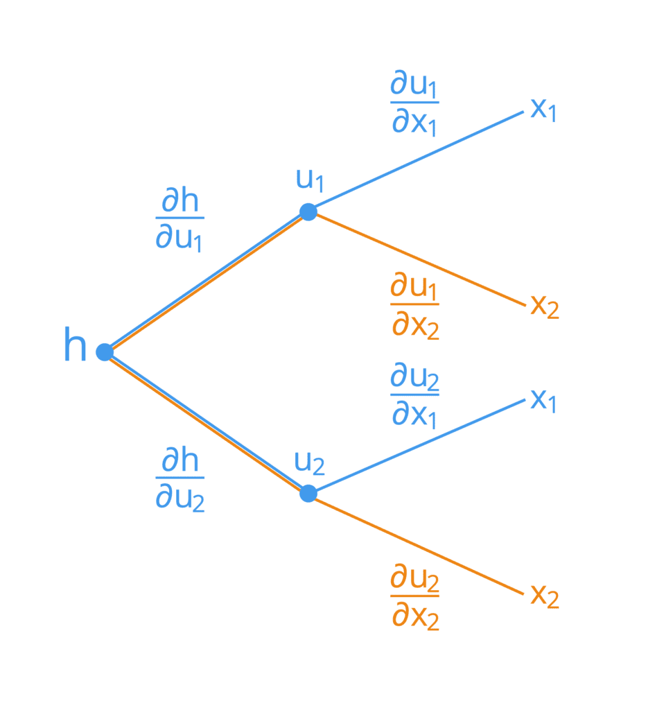
Suppose

$$h=h(u_1,u_2),$$

where both $u_1$ and $u_2$ depend on $x_1$ and $x_2$. Then the multivariable chain rule gives

$$\frac{\partial h}{\partial x_1}=\frac{\partial h}{\partial u_1}\frac{\partial u_1}{\partial x_1}+\frac{\partial h}{\partial u_2}\frac{\partial u_2}{\partial x_1}.$$

Similarly,

$$\frac{\partial h}{\partial x_2}=\frac{\partial h}{\partial u_1}\frac{\partial u_1}{\partial x_2}+\frac{\partial h}{\partial u_2}\frac{\partial u_2}{\partial x_2}.$$

The two products in each equation correspond to the two distinct dependency paths in the computational graph.

Worked branching example

Let

$$u_1=x_1+x_2,$$ $$u_2=x_1{x}_2,$$

and let the final scalar output be

$$h=u_1^2+3u_2.$$

First calculate the local derivatives of the output with respect to its two immediate inputs:

$$\frac{\partial h}{\partial u_1}=2u_1,$$ $$\frac{\partial h}{\partial u_2}=3.$$

Now calculate how the intermediates depend on $x_1$:

$$\frac{\partial u_1}{\partial x_1}=1,$$ $$\frac{\partial u_2}{\partial x_1}=x_2.$$

Apply the multivariable chain rule:

$$\frac{\partial h}{\partial x_1}=(2u_1)(1)+(3)(x_2).$$

At

$$(x_1,x_2)=(2,4),$$

the intermediate value is

$$u_1=2+4=6.$$

Therefore,

$$\frac{\partial h}{\partial x_1}=2(6)+3(4)=24.$$

The interpretation is precise: near this input point, a small increase in $x_1$, with $x_2$ held fixed, increases $h$ at a local rate of about $24$. That total rate includes both effects: the effect through $u_1$ and the separate effect through $u_2$.

This “multiply within a path, add across paths” rule is the structural idea behind reverse-mode automatic differentiation.

---

A miniature model-loss chain

Consider a one-feature prediction model:

$$z=wx+b,$$

where $w$ and $b$ are parameters, $x$ is an input feature, and $z$ is the prediction. For one labeled example with target $t$, define squared error:

$$L=(z-t{)}^2.$$

This is a small version of the structure used in machine learning: parameters affect a prediction, which affects a loss.

To find the sensitivity of loss to the weight $w$, treat $z$ as the intermediate variable:

$$\frac{\partial L}{\partial w}=\frac{\partial L}{\partial z}\frac{\partial z}{\partial w}.$$

The local derivatives are

$$\frac{\partial L}{\partial z}=2(z-t),$$

and

$$\frac{\partial z}{\partial w}=x.$$

Thus,

$$\frac{\partial L}{\partial w}=2(z-t)x.$$

For the bias,

$$\frac{\partial z}{\partial b}=1,$$

so

$$\frac{\partial L}{\partial b}=2(z-t).$$

The difference between these gradients comes entirely from the local dependency of $z$ on each parameter. The weight affects the prediction in proportion to $x$; the bias affects it by the same amount regardless of $x$.

A speech model is vastly larger than this toy calculation: its inputs are feature tensors or audio representations, its parameters are matrices, and its computation graph has many layers. But the same local logic applies. Frameworks such as PyTorch record a graph of operations and use the chain rule to calculate parameter gradients without manually expanding an enormous expression.

---

Chain-rule error checks

Before trusting a derivative, inspect it with these checks:

Check	What it catches
Identify the outermost operation first.	Misidentifying a nested expression as a product.
Keep the original inside expression in the outer derivative.	Writing $f^{\prime }(x)$ when the correct term is $f^{\prime }(g(x))$.
Include one local derivative for every stage.	Forgetting the derivative of an inner function.
Multiply along one dependency path.	Omitting a local sensitivity factor.
Add contributions from distinct paths.	Missing a second way an input influences the output.
Check the derivative’s shape.	In ML, the gradient with respect to a parameter must have that parameter’s shape.

For hand calculations, naming intermediate variables is more than a stylistic preference. It turns a complicated expression into a short computation graph, makes the dependencies explicit, and mirrors the reasoning used by automatic differentiation systems.

---

Key takeaways

• The chain rule differentiates a composition such as $f(g(x))$:

$$\frac{d}{dx}f(g(x))=f^{\prime }(g(x))g^{\prime }(x).$$

• Differentiate the outer function first, evaluate it at the unchanged inner expression, and multiply by the derivative of the inner function.
• For several nested stages, multiply the local derivatives for all stages.
• In a branching computation graph, multiply local derivatives along each path and add the contributions across paths.
• Backpropagation is a scalable implementation of this rule for the large computation graphs used in neural networks.

Next, the course shifts from local change in functions to numerical summaries of data: mean, variance, and covariance. Those statistics will become essential when inspecting speech features, dataset balance, and variation across speakers or recording conditions.