Sensor Fusion for Robust Orientation and Activity Detection

Hello! Let's continue our exploration of motion analysis.

In our last lesson, we examined the inner workings of accelerometers and gyroscopes. We concluded that they are a perfect team: the accelerometer provides a stable, long-term sense of "down" using gravity but is noisy, while the gyroscope gives clean, responsive rotation data but drifts over time. We ended with the question: how do we get the best of both worlds?

This lesson directly answers that question. Our learning outcome is to apply sensor fusion techniques to combine data from multiple motion sensors for robust orientation and activity detection. We'll move from the individual sensor principles to the algorithms that intelligently merge their data streams. This is the key to transforming raw sensor outputs into a reliable understanding of movement, which is essential for your work at Neuraease in distinguishing emotional states from physical activity.

1. The Case for Fusion: Why Single Sensors Fail

Before diving into the algorithms, let's solidify our understanding of why we must fuse sensor data. Each sensor in an Inertial Measurement Unit (IMU)—accelerometer, gyroscope, and often a magnetometer—has a critical flaw when used alone for orientation tracking.

To summarize the key challenges:

• Accelerometer: It measures both motion and gravity. During fast movements, the motion component can overwhelm the gravity vector, making tilt estimation unreliable. Furthermore, it cannot measure rotation around the vertical axis (yaw or heading) at all.
• Gyroscope: Its integration process (summing up angular velocities over time) accumulates small errors, leading to drift. Over minutes, or even seconds, its orientation estimate will diverge from reality.
• Magnetometer: It provides an absolute heading (like a compass), which is great for correcting yaw drift. However, it's highly susceptible to magnetic interference from nearby metals (soft iron distortion) or objects that generate their own fields like motors or electronics (hard iron distortion).

Clearly, to get a stable and accurate 3D orientation, we need a method that combines the gyroscope's responsiveness, the accelerometer's long-term tilt stability, and the magnetometer's absolute heading reference. This method is sensor fusion.

2. The Core Idea: An Intelligent Blending

Sensor fusion isn't just a simple average. It's a "fancy average" where we dynamically decide how much to trust each sensor at any given moment. Let's watch a video that provides a great conceptual overview of this blending process.

The video introduces the central idea: we primarily rely on the integrated gyroscope data for a smooth, continuous orientation estimate. Simultaneously, we use the accelerometer and magnetometer data as a slow, steady "correction force" to pull the gyroscope's estimate back on track and prevent it from drifting away.

Now, let's look at the specific algorithms that implement this "fancy averaging."

3. Sensor Fusion Algorithms

There are several algorithms for sensor fusion, ranging from simple and computationally cheap to complex and highly robust. We'll focus on the three most common categories.

a) The Complementary Filter

This is the most straightforward approach. It combines a high-pass filtered version of the gyroscope data with a low-pass filtered version of the accelerometer/magnetometer data.

Conceptually, this makes sense:

• Gyroscope: We trust its fast changes (high-frequency), but not its slow drift (low-frequency). A high-pass filter achieves this.
• Accelerometer/Magnetometer: We trust its long-term average (low-frequency) to define "down" and "north", but not its fast, noisy jitter (high-frequency). A low-pass filter achieves this.

In its simplest form, it's implemented as a weighted sum:

${\text{angle}}_{\text{new}}=\alpha \cdot ({\text{angle}}_{\text{gyro}})+(1-\alpha )\cdot ({\text{angle}}_{\text{accel/mag}})$

Here, angle_gyro is the previous angle updated with the new gyroscope reading, and angle_accel/mag is the angle calculated directly from the accelerometer and magnetometer. The weighting factor $\alpha$ is typically set high (e.g., 0.98), meaning we trust the gyroscope about 98% and use the accelerometer/magnetometer for a 2% correction in each step.

• Pros: Simple to implement, computationally very efficient (great for low-power microcontrollers).
• Cons: The weighting factor $\alpha$ is fixed. It can't adapt if, for example, the accelerometer suddenly becomes very noisy during a high-impact event.

b) The Kalman Filter

The Kalman filter is a much more powerful and adaptive approach. It's a cornerstone of modern control theory and robotics. Given your ECE background, you may recall it from courses on control systems or signal processing.

Instead of a fixed weight, the Kalman filter dynamically calculates the optimal weight (called the Kalman Gain) at each time step based on the uncertainty of its estimates.

The process, simplified, is a two-step loop:

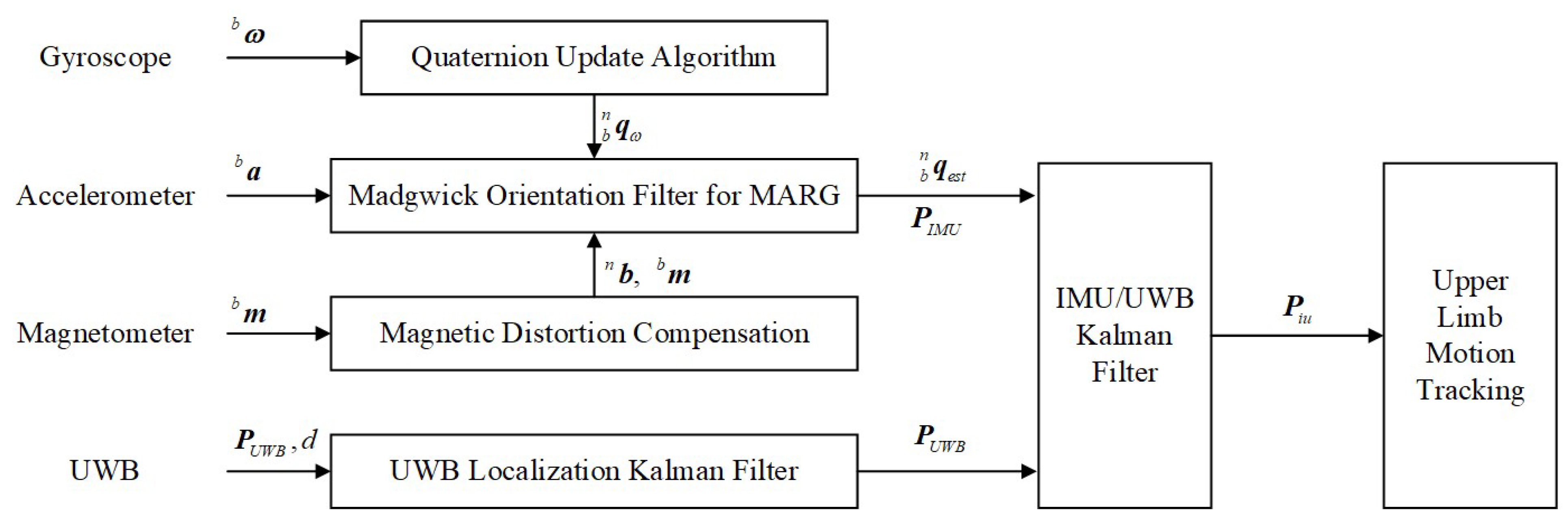
1. Predict: The filter uses a model of the system's physics (in this case, rotational kinematics) to predict what the new orientation should be based on the gyroscope reading. With this prediction comes an estimate of its uncertainty, which grows in this step because we know gyros drift.
2. Update: The filter takes a new measurement from the accelerometer and magnetometer. It compares this measurement to its prediction. Based on how noisy it thinks the measurement is versus how uncertain its prediction is, it computes the Kalman Gain and makes a correction. If the measurement is trusted, the correction is large. If the prediction is trusted, the correction is small.

• Pros: Highly accurate and adaptive. It provides the statistically optimal estimate if the system and noise are modeled correctly.
• Cons: Mathematically complex and computationally more expensive than a complementary filter. The standard Kalman filter assumes linear systems, so for 3D orientation (which is non-linear), a variant called an Extended Kalman Filter (EKF) is typically used.

c) Madgwick and Mahony Filters

These are more recent algorithms that have become very popular in embedded systems. They offer a performance level close to a Kalman filter but are computationally much cheaper.

They use a different mathematical representation for orientation called quaternions (a four-dimensional number system that avoids some problems of Euler angles like gimbal lock) and an optimization technique called gradient descent to minimize the error between the orientation estimated from the gyroscope and the orientation determined by the accelerometer/magnetometer.

You are likely to encounter these filters implemented in libraries for IMU sensors, so it's good to know what they are.

Test your understanding!

You are designing a simple wearable device on a very low-power microcontroller to detect if a person is generally active or sedentary throughout the day. Extreme accuracy is not the main goal, but battery life is critical. Which sensor fusion algorithm would you choose and why?

Show answer

A Complementary Filter would be the most suitable choice. It is computationally very cheap, which directly translates to lower power consumption and longer battery life. While not as robust as a Kalman filter, its performance is often "good enough" for basic activity detection where you are distinguishing between large-scale states like sitting, walking, or running, rather than needing precise joint-angle kinematics.

4. From Orientation to Activity

Once you have a robust stream of orientation data (roll, pitch, yaw) from your fusion algorithm, you can begin to analyze activity.

• Activity Classification: You can use the orientation and raw acceleration data as features for a machine learning model to classify activities like sitting, standing, walking, or running. For your startup, this could be the first step in differentiating "anxious pacing" from "taking a walk."
• Movement Quantification: You can calculate metrics like the total angular distance traveled, the smoothness of movement, or the number of posture transitions in a given time. This can provide insight into restlessness or motor agitation.

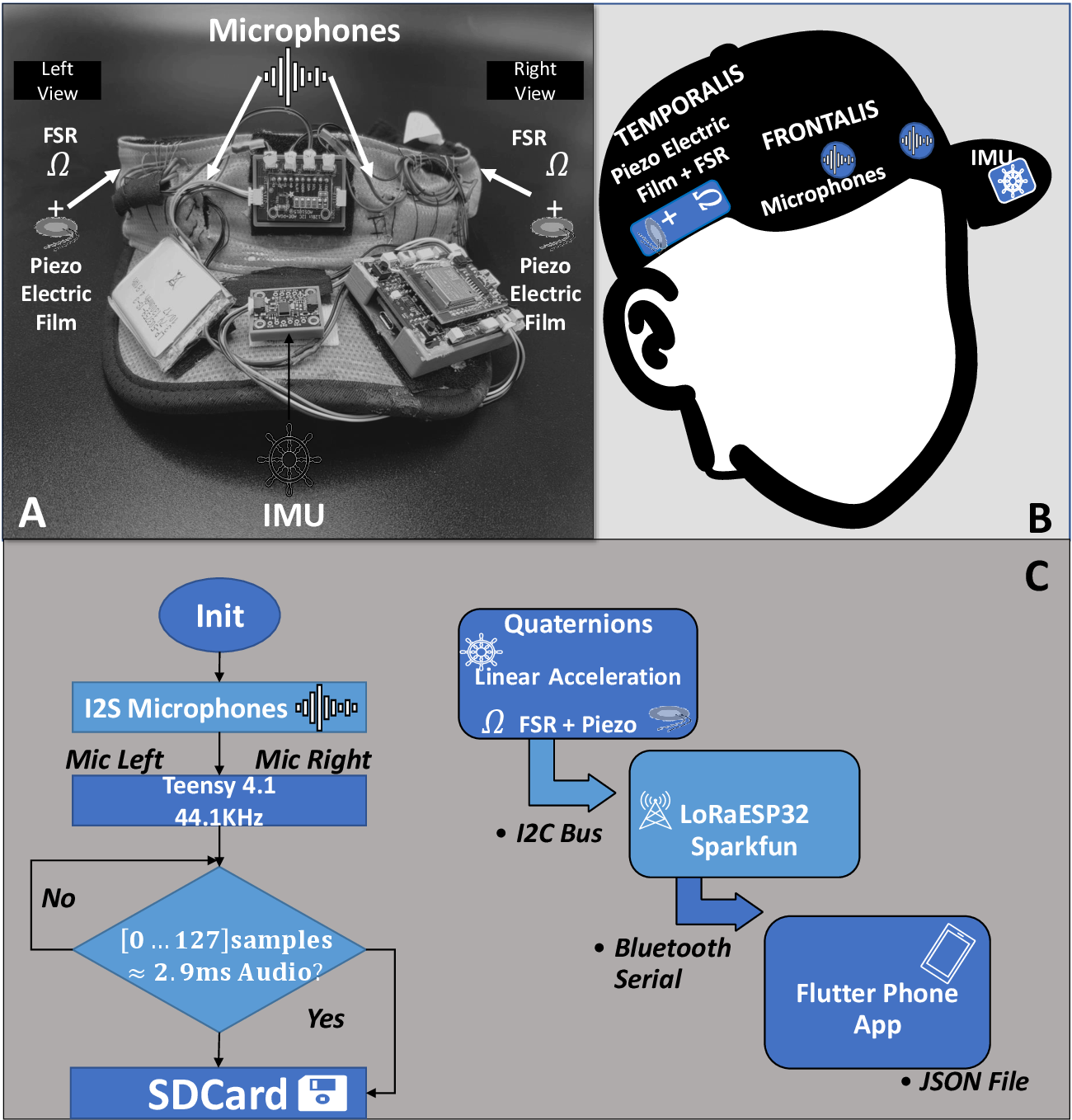
The image below shows how an IMU fits into a larger multi-modal system, just like the one you are envisioning for Neuraease. The IMU provides the crucial motion context for interpreting all the other physiological signals.

Conclusion

In this lesson, we bridged the gap between individual motion sensors and a meaningful understanding of movement. We've seen that robust orientation tracking is not possible with any single sensor, but requires an intelligent fusion of their complementary strengths.

Key Takeaways:

• Sensor Fusion is necessary to overcome the individual weaknesses of accelerometers (noise, no yaw), gyroscopes (drift), and magnetometers (magnetic interference).
• The Complementary Filter is a simple, efficient algorithm that uses a fixed weighted average to combine sensor data. It's great for low-power applications.
• The Kalman Filter is a more complex, adaptive algorithm that uses a predictive model and dynamically adjusts its weights based on estimated uncertainty, providing optimal accuracy.
• Madgwick/Mahony filters are modern, computationally efficient alternatives to Kalman filters, often used in embedded systems.
• The output of a fusion algorithm—a stable 3D orientation—is the foundation for higher-level activity detection and behavioral analysis.

Preview of the Next Lesson:
With a solid grasp of how to measure orientation, we can now focus on specific motor behaviors. In our next lesson, we will explore how to design an instrumentation setup to measure motor responses, such as reaction time and fine movement patterns, and discuss methods for analyzing behavioral patterns from the continuous data streams our wearables can generate.