Audio Waveforms: Visualization and Basic Time-Domain Operations

Hello! Welcome to the seventh lesson in our "Foundations of Digital Audio" module.

In our previous lesson, we successfully bridged the gap between audio files on disk and the numerical world of PyTorch. You learned how to use torchaudio.load() to decode audio into a waveform tensor and a sample_rate, the fundamental representation for all our future work.

Now that we have this raw data in hand, what can we learn from it? This lesson dives into the time domain. Our goal is to visualize and interpret audio waveforms and perform basic time-domain operations like trimming and concatenation. You'll learn to "read" an audio signal visually and manipulate it directly using PyTorch's tensor operations, a foundational skill for audio data preparation and analysis.

---

1. The Waveform: A Picture of Sound

An audio waveform is the most fundamental visual representation of sound. It's a graph that plots the change in amplitude (related to air pressure) over time.

Before we dive into code, let's build a solid conceptual understanding. The following reading explains how a simple two-dimensional plot can represent the complex phenomenon of a sound wave.

As the text explains, the horizontal axis is time, and the vertical axis is amplitude.

• A flat line at zero represents silence (no change in pressure).
• The peaks and troughs represent the intensity of the pressure changes.

Let's see what this looks like in code.

2. Visualizing Waveforms with Python

Now that we know how to load a waveform tensor with torchaudio, we can use matplotlib to plot it. The tensor's shape, as you'll recall, is [channels, samples].

Here's a basic workflow:

1. Load the audio file using torchaudio.load().
2. Create a time axis by dividing the sample indices by the sample rate.
3. Use matplotlib.pyplot.plot() to graph amplitude against time.

import torch
import torchaudio
import matplotlib.pyplot as plt




# Let's use a sample audio file from torchaudio's dataset for reproducibility
# This downloads a small dataset.
from torchaudio.datasets import SPEECHCOMMANDS
dataset = SPEECHCOMMANDS(root=".", download=True)
waveform, sample_rate, _, _, _ = dataset[0] # Get the first sample

print(f"Waveform shape: {waveform.shape}")
print(f"Sample rate: {sample_rate} Hz")

def plot_waveform(waveform, sample_rate, title="Waveform"):
    """Plots the waveform of a given audio tensor."""
    num_channels, num_frames = waveform.shape
    time_axis = torch.arange(0, num_frames) / sample_rate

    figure, axes = plt.subplots(num_channels, 1)
    if num_channels == 1:
        axes = [axes]
    for c in range(num_channels):
        axes[c].plot(time_axis, waveform[c].numpy())
        axes[c].set_ylabel(f"Channel {c+1}")
        axes[c].set_xlim([0, time_axis[-1]])
    figure.suptitle(title)
    plt.xlabel("Time (seconds)")
    plt.tight_layout()
    plt.show()

plot_waveform(waveform, sample_rate)

The output of this code will be a plot showing the amplitude of the spoken word over its one-second duration.

The following video provides a live demonstration of loading and plotting, reinforcing what we've just done.

3. Interpreting the Waveform: From Squiggles to Meaning

A raw waveform plot can tell you a surprising amount about the audio signal.

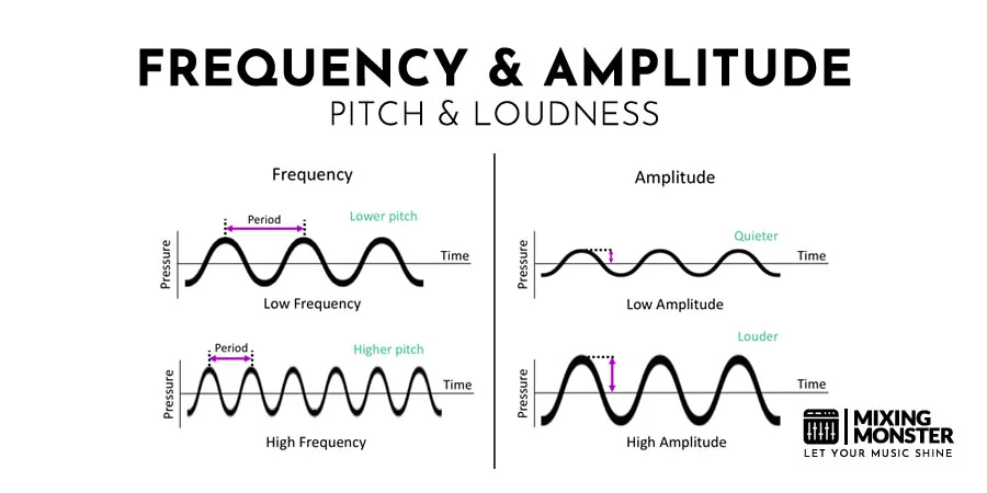
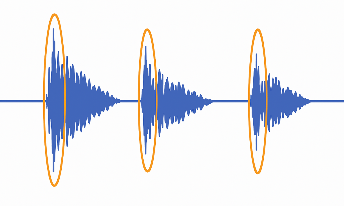
When you look at a waveform, here are key features to look for:

• Silence vs. Sound: Long, flat sections near the zero-amplitude line indicate silence. Bursts of activity indicate sound events.
• Transients: These are the initial, high-energy spikes at the very beginning of a sound, like a drum hit or a consonant in speech. They are often the loudest part of the sound event.
• Sustain and Decay: Following a transient, the amplitude might hold steady (sustain) and then gradually decrease (decay).
• Clipping: If the waveform looks "squared off" at the top or bottom (at +1.0 or -1.0), it means the signal was too loud during recording and was clipped. This is a form of distortion that results in information loss.

By zooming in, as shown in the video, you can inspect the periodic nature of the wave. A tighter, more frequent pattern indicates a higher-pitched sound, while a slower, wider pattern indicates a lower-pitched one.

4. Time-Domain Operations in PyTorch

Since our waveform is a PyTorch tensor, we can use standard tensor operations to manipulate it. This is far more efficient than saving and re-loading files with ffmpeg for simple modifications.

Trimming and Slicing

The simplest way to trim audio is to slice the tensor. If you want to extract a segment from 0.25 to 0.75 seconds, you can calculate the corresponding sample indices and slice.

# Continuing from the previous code block
start_time = 0.25
end_time = 0.75

start_sample = int(start_time * sample_rate)
end_sample = int(end_time * sample_rate)

trimmed_waveform = waveform[:, start_sample:end_sample]

plot_waveform(trimmed_waveform, sample_rate, title="Trimmed Waveform (0.25s - 0.75s)")

Padding

Often, you need all audio clips in a batch to have the same length for model training. If a clip is too short, you can pad it with zeros. torch.nn.functional.pad is perfect for this.

The following reading explains how to create a versatile function for both padding and trimming to a fixed length.

Let's implement a simplified version of this idea. We'll pad our trimmed waveform to be 1 second long.

target_length_seconds = 1.0
target_length_samples = int(target_length_seconds * sample_rate)

current_length_samples = trimmed_waveform.shape[1]




# The pad function takes a tuple of (pad_left, pad_right)
# We only want to pad at the end.
padding_needed = target_length_samples - current_length_samples




# Ensure we don't pad if it's already long enough
if padding_needed > 0:
    padded_waveform = torch.nn.functional.pad(trimmed_waveform, (0, padding_needed))
else:
    padded_waveform = trimmed_waveform # Or trim if it was too long

plot_waveform(padded_waveform, sample_rate, title="Padded to 1 second")

print(f"Original trimmed length: {current_length_samples} samples")
print(f"Padded length: {padded_waveform.shape[1]} samples")

Concatenation

To join two audio clips, you can use torch.cat(). The key is to ensure they have the same sample rate and number of channels. You concatenate along dim=1 (the time/samples dimension).

# Let's get another audio clip
waveform2, sample_rate2, _, _, _ = dataset[1]




# For a robust system, you'd assert sample_rate == sample_rate2
# and resample if necessary. For now, we assume they match.

concatenated_waveform = torch.cat([padded_waveform, waveform2], dim=1)

plot_waveform(concatenated_waveform, sample_rate, title="Concatenated Waveform")

This simple operation is the basis for creating longer audio streams from smaller segments or for data augmentation techniques where you might splice different audio events together.

---

Conclusion

In this lesson, you've learned to treat the audio waveform not just as an abstract concept but as a concrete torch.Tensor that you can see and manipulate.

Key Takeaways:

• A waveform plot shows amplitude versus time, providing a visual signature of a sound.
• By inspecting a waveform, you can identify key characteristics like silence, sound events, transients, and potential clipping.
• Basic time-domain operations are efficient tensor manipulations in PyTorch:
  • Trimming: Slicing the tensor along its time dimension (waveform[:, start:end]).
  • Padding: Using torch.nn.functional.pad() to add values (usually zeros) to match a target length.
  • Concatenation: Using torch.cat([...], dim=1) to join waveforms end-to-end.

You now have the skills to load, visualize, and perform fundamental manipulations on raw audio data. However, the raw amplitude values are often not ideal for direct use in machine learning models. In our next lesson, we will address this by learning how to apply various audio normalization techniques (peak, RMS, LUFS) to standardize the loudness of our audio clips, a crucial step for robust model training.