Audio Normalization Techniques and Use Cases

Hello! Welcome to the final lesson of our first module, "Foundations of Digital Audio."

In our last session, you mastered the art of representing audio as PyTorch tensors. You learned to visualize waveforms and perform fundamental time-domain manipulations like trimming and concatenation. We concluded by noting that raw amplitude values can be inconsistent, which poses a problem for training robust machine learning models.

This lesson directly addresses that challenge. Our learning outcome is to apply various audio normalization techniques (peak, RMS, LUFS) and explain their use cases. We will explore why simply preventing digital clipping isn't enough and how we can standardize audio volume in a way that aligns with human perception—a critical step for preparing high-quality datasets for tasks like speech recognition and text-to-speech.

1. The Need for Normalization

Imagine training a speech recognition model. If some audio files in your dataset are very quiet and others are extremely loud, the model might struggle. It could incorrectly associate loudness with a particular word or speaker, or its training process might become unstable due to the wide variation in input data magnitude.

Normalization is the process of adjusting the volume of audio clips to a standard level. This ensures consistency across a dataset, leading to more stable training and better model performance. However, as we'll see, "volume" can be defined in several ways.

Let's begin by exploring why the most straightforward approach, peak normalization, is often insufficient.

As the video demonstrates, our ears don't perceive loudness based on signal peaks alone. Loudness is a subjective, perceptual phenomenon that is heavily influenced by frequency content and signal duration. Let's break down the three main normalization techniques that address this in different ways.

2. Peak Normalization

Peak normalization is the simplest method. It adjusts the signal's gain so that its highest peak reaches a target level, typically 0 dBFS (Decibels relative to Full Scale). For a floating-point waveform where the maximum possible amplitude is 1.0, this means scaling the waveform so its maximum absolute value is 1.0.

The Math: dBFS and Peak Scaling

Decibels (dB) represent a logarithmic ratio. In the digital domain, dBFS measures the amplitude of a signal compared to the maximum possible level a system can handle before clipping.

For a floating-point signal $x$ in the range $[-1,1]$, the full scale reference is 1.0. The peak level in dBFS is calculated as:

To perform peak normalization to a target_dbfs level, you first convert the target from the logarithmic dB scale to a linear amplitude scale:

Then, you calculate the necessary gain and apply it:

• Use Case: Primarily to prevent clipping and maximize the signal-to-noise ratio by using the full available bit depth.
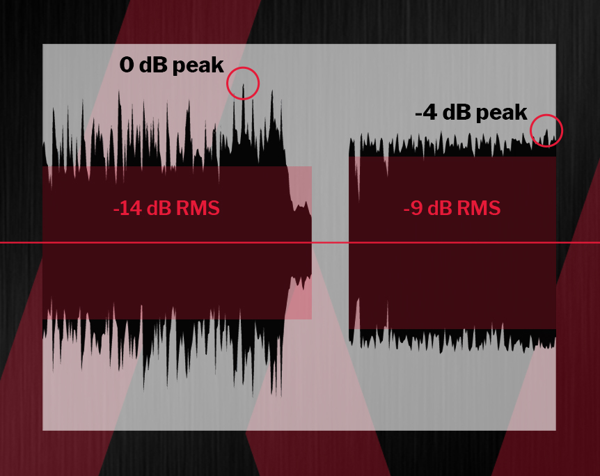
• Drawback: As seen in the video, it has a poor correlation with perceived loudness. A file with one loud drum hit and quiet speech will be normalized based on the drum hit, making the speech potentially inaudible.

3. RMS Normalization

A better proxy for loudness is the Root Mean Square (RMS) amplitude. RMS measures the average power of the signal over time, giving a more stable representation of its overall energy level.

The Math: RMS Calculation

The RMS of a signal $x$ with $N$ samples is calculated by squaring all amplitude values, taking the mean, and then taking the square root.

The formula is:

The process for RMS normalization is similar to peak normalization: calculate the current RMS level, determine the gain needed to reach a target RMS level, and apply it to the signal.

• Use Case: Common in speech processing pipelines to ensure that different speakers or recordings have a similar average volume. It's a significant improvement over peak normalization for standardizing perceived loudness.
• Drawback: While better, RMS is still "agnostic" to frequency. The human ear is not equally sensitive to all frequencies. An audio clip with high energy in the low bass will have a high RMS value but might not sound as loud as a clip with the same RMS value concentrated in the mid-range, where our hearing is most sensitive.

4. Loudness Normalization (LUFS / LKFS)

To solve the shortcomings of peak and RMS, the broadcasting and music industries developed a standard that measures loudness in a way that models human perception. This is specified in the ITU-R BS.1770 standard.

The unit of measurement is LUFS (Loudness Units relative to Full Scale) or LKFS (Loudness, K-weighted, relative to Full Scale) — they are identical.

This method involves two key steps that RMS normalization lacks:

1. K-Weighting: A frequency-weighting filter is applied to the signal before measuring its power. This filter de-emphasizes low frequencies and boosts upper-mid frequencies (around 2-5 kHz), crudely approximating the non-linear sensitivity of the human ear.
2. Gating: A sophisticated gating mechanism is used to exclude quiet parts of the signal (e.g., long pauses) from the integrated loudness measurement. This ensures the measurement reflects the loudness of the "foreground" content, not the average loudness diluted by silence.

Finally, let's hear the difference. The following clip plays a sequence of audio clips first normalized by peak, then by loudness.

• Use Case: The gold standard for audio delivery on platforms like YouTube, Spotify, and in broadcasting. It is the most perceptually accurate method and is highly recommended for preparing datasets for generative models like TTS, where consistent perceived loudness is crucial for output quality.
• Drawback: More computationally expensive than peak or RMS. Implementing it from scratch is complex, so we rely on specialized libraries.

5. Practical Implementation in Python

Let's apply these three techniques. For LUFS, we will use the pyloudnorm library, which is a Python implementation of the ITU-R BS.1770-4 standard.

First, make sure you have it installed:
pip install pyloudnorm numpy

Here is a Python script demonstrating how to implement each normalization function.

import torch
import torchaudio
import numpy as np
import pyloudnorm as pyln




# --- Helper Functions ---
def to_db(value, reference=1.0):
    """Convert a linear value to dB."""
    return 20 * np.log10(value / reference)

def from_db(db_value):
    """Convert a dB value to linear."""
    return 10 ** (db_value / 20)




# --- Load Sample Audio ---
# We'll use the same sample from the previous lesson
from torchaudio.datasets import SPEECHCOMMANDS
dataset = SPEECHCOMMANDS(root=".", download=True)
waveform, sample_rate, _, _, _ = dataset[0]
signal = waveform.numpy().squeeze() # Use numpy for easier calculations

print(f"Original Signal Stats:")
print(f"  - Peak: {np.max(np.abs(signal)):.4f} linear, {to_db(np.max(np.abs(signal))):.2f} dBFS")
rms = np.sqrt(np.mean(signal**2))
print(f"  - RMS: {rms:.4f} linear, {to_db(rms):.2f} dBFS")
meter = pyln.Meter(sample_rate)
loudness = meter.integrated_loudness(signal)
print(f"  - LUFS: {loudness:.2f} LUFS")




# --- Normalization Functions ---

def normalize_peak(signal, target_dbfs=-0.1):
    """Normalize the signal to a target peak dBFS level."""
    target_linear = from_db(target_dbfs)
    current_peak = np.max(np.abs(signal))
    if current_peak == 0: return signal # Avoid division by zero
    gain = target_linear / current_peak
    return signal * gain

def normalize_rms(signal, target_dbfs=-20.0):
    """Normalize the signal to a target RMS dBFS level."""
    target_linear = from_db(target_dbfs)
    current_rms = np.sqrt(np.mean(signal**2))
    if current_rms == 0: return signal
    gain = target_linear / current_rms
    return signal * gain

def normalize_lufs(signal, sample_rate, target_lufs=-23.0):
    """Normalize the signal to a target integrated loudness (LUFS)."""
    meter = pyln.Meter(sample_rate)
    current_lufs = meter.integrated_loudness(signal)
    gain_db = target_lufs - current_lufs
    gain_linear = from_db(gain_db)
    return signal * gain_linear




# --- Apply and Compare ---
peak_norm_signal = normalize_peak(signal, target_dbfs=-1.0)
rms_norm_signal = normalize_rms(signal, target_dbfs=-23.0)
lufs_norm_signal = normalize_lufs(signal, sample_rate, target_lufs=-23.0)

print("\n--- After Normalization ---")




# Peak Normalized
print(f"Peak Normalized (Target -1.0 dBFS):")
print(f"  - New Peak: {to_db(np.max(np.abs(peak_norm_signal))):.2f} dBFS")
print(f"  - New LUFS: {pyln.Meter(sample_rate).integrated_loudness(peak_norm_signal):.2f} LUFS")




# RMS Normalized
print(f"RMS Normalized (Target -23.0 dBFS):")
new_rms = np.sqrt(np.mean(rms_norm_signal**2))
print(f"  - New RMS: {to_db(new_rms):.2f} dBFS")
print(f"  - New Peak: {to_db(np.max(np.abs(rms_norm_signal))):.2f} dBFS") # Check for clipping!
if np.max(np.abs(rms_norm_signal)) > 1.0:
    print("    -> WARNING: Signal is clipping!")




# LUFS Normalized
print(f"LUFS Normalized (Target -23.0 LUFS):")
print(f"  - New LUFS: {pyln.Meter(sample_rate).integrated_loudness(lufs_norm_signal):.2f} LUFS")
print(f"  - New Peak: {to_db(np.max(np.abs(lufs_norm_signal))):.2f} dBFS")
if np.max(np.abs(lufs_norm_signal)) > 1.0:
    print("    -> WARNING: Signal is clipping!")

When you run this code, pay close attention to the "New Peak" values after RMS and LUFS normalization. It's common for these methods to push the signal's peaks above 0 dBFS, causing clipping. In practice, after RMS or LUFS normalization, you often apply a limiter—a type of dynamic range compressor—to bring down the peaks without affecting the overall perceived loudness. We will not cover limiters in this course, but it is important to be aware of this potential issue.

Conclusion

You have now completed the "Foundations of Digital Audio" module! This final lesson armed you with the theory and practical skills to standardize audio volume, a critical preprocessing step.

Key Takeaways:

• Normalization is crucial for creating consistent datasets and ensuring stable model training.
• Peak Normalization is simple and prevents clipping but does not correlate well with perceived loudness.
• RMS Normalization measures the average power of a signal and is a better, though imperfect, proxy for loudness.
• LUFS Normalization (ITU-R BS.1770) is the industry standard that uses frequency weighting (K-weighting) and gating to provide a perceptually accurate measure of loudness. It is the recommended method for most modern audio ML applications.
• When normalizing to RMS or LUFS, you must be mindful of potential clipping and may need to apply a limiter as a final step.

With this foundation, you are ready to move from the time domain to the frequency domain. In our next module, "Spectral Analysis of Audio Signals," we will begin with one of the most important tools in all of signal processing: the Fourier Transform. This will allow us to decompose a signal into its constituent frequencies and build the powerful visual representations, like spectrograms, that serve as the input to almost all modern audio AI systems.