Loading Audio in PyTorch with torchaudio

Hello! Welcome to the sixth lesson in our "Foundations of Digital Audio" module.

In our last lesson, you mastered ffmpeg, the essential command-line tool for preparing audio files—converting formats, resampling, and changing channel layouts. Those operations happen at the file level, getting your data ready on disk.

Today, we take the crucial next step: bringing that data into your code. To train a neural network, you need to represent audio as a numerical tensor. This lesson focuses on how to load, decode, and represent audio tensors in PyTorch using torchaudio's I/O backends. We will bridge the gap between files on your hard drive and the tensors your PyTorch models can process.

Given your background in PyTorch and building ML systems, we won't just look at loading a single file. We will also see how these I/O functions form the backbone of a robust data loading pipeline using PyTorch's Dataset class, a pattern essential for any serious project.

1. Introducing torchaudio

torchaudio is the official PyTorch library for audio processing. It integrates seamlessly with PyTorch tensors and provides utilities for I/O, data augmentation, feature extraction, and even pre-trained models. While ffmpeg is a general-purpose tool, torchaudio is specifically designed for the PyTorch ecosystem, making it the standard choice for audio AI research and development within this framework.

Let's begin by seeing how to get information about an audio file and load it into our environment.

As the video demonstrates, the core I/O operations are straightforward. Let's formalize them.

torchaudio.info()

This function lets you peek inside an audio file without loading the entire thing into memory. It returns a metadata object containing key information.

import torch
import torchaudio




# Assume we have a file 'audio.wav'
# You can use a file you prepared from the previous lesson
filepath = "output_16k_mono.wav" 

metadata = torchaudio.info(filepath)
print(metadata)




# Expected output might look like this:
# AudioMetaData(sample_rate=16000, num_frames=80000, num_channels=1, bits_per_sample=16, encoding='PCM_S')

This is the programmatic equivalent of running ffprobe and is an essential first step for validating your audio data.

torchaudio.load()

This is the workhorse function. It decodes an audio file and returns its contents as a PyTorch tensor.

waveform, sample_rate = torchaudio.load(filepath)

print(f"Waveform shape: {waveform.shape}")
print(f"Sample rate: {sample_rate}")
print(f"Waveform dtype: {waveform.dtype}")
print(f"Waveform value range: min={waveform.min()}, max={waveform.max()}")

2. The Waveform Tensor: The Foundation of Audio AI

The waveform tensor returned by torchaudio.load() is the fundamental object you'll be working with. Understanding its structure is critical.

Let's break down its properties based on the code output above:

• Shape: The tensor has a shape of [num_channels, num_frames] (or [C, L]). This is a standard convention in torchaudio.
  • num_channels: The first dimension. 1 for mono, 2 for stereo.
  • num_frames: The second dimension, also called length. This is the total number of individual samples in the audio clip. For a 5-second clip at 16,000 Hz, this will be $5\times 16000=80000$ samples.
• Data Type (dtype): It is typically torch.float32.
• Value Range: The sample values are normalized to be within the range [-1.0, 1.0]. torchaudio handles the conversion from the file's native format (e.g., 16-bit integers ranging from -32768 to 32767) to this floating-point representation.

The following reading provides a clear text-based explanation of the audio tensor.

3. Under the Hood: I/O Backends

How does torchaudio actually read all those different file formats? It doesn't implement the decoders itself. Instead, it uses a pluggable system of I/O backends—underlying libraries that do the heavy lifting. The main backends are:

• soundfile: A high-performance library based on libsndfile. It's excellent for standard formats like WAV and FLAC.
• sox_io: A backend that uses the SoX library. It has broad format support but can sometimes be slower.
• ffmpeg: A backend that uses the same ffmpeg library you learned about in the last lesson. It offers the widest possible format support, including compressed formats like MP3 and AAC, and audio from video containers.

The availability of these backends depends on your operating system and how torchaudio was installed. You can check which are available and which is currently active:

print("Available backends:", torchaudio.list_audio_backends())
print("Current backend:", torchaudio.get_audio_backend())

For most common uncompressed formats, soundfile is often the fastest. Your choice of backend can have a significant impact on data loading speed, which becomes critical when training on huge datasets.

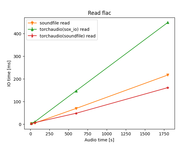
Since you have experience with ffmpeg and are aiming for robust systems, it's good to know that the ffmpeg backend for torchaudio provides maximum compatibility. You can explicitly set the backend if needed: torchaudio.set_audio_backend("ffmpeg").

4. Advanced and Efficient Loading

torchaudio.load() has more capabilities that are useful for building efficient pipelines.

Loading a Section of a File

Instead of loading an entire large file into memory and then slicing the tensor, you can tell torchaudio to only decode a specific chunk. This is done with the frame_offset and num_frames arguments. This is much more memory and I/O efficient.

This is especially useful for training, where you might want to load random chunks from long audio files for data augmentation.

5. Practical Application: A Custom PyTorch Dataset

Loading a single file is a good start, but in a real project, you'll be working with thousands. The standard PyTorch paradigm for this is to create a custom Dataset class. This class is responsible for telling PyTorch how many items are in your dataset (__len__) and how to get a single item given an index (__getitem__).

This is where torchaudio.load() truly shines. You call it inside the __getitem__ method to load and return one audio sample on demand. This pattern is fundamental to building scalable audio data pipelines.

Building a Dataset class like this allows PyTorch's DataLoader to handle multi-processing, shuffling, and batching automatically, dramatically speeding up your training loop. This is a core competency for any AI engineer or researcher.

Conclusion

In this lesson, you've learned how to bring audio data to life inside PyTorch. You've moved beyond file manipulation on the command line to creating the fundamental data structure for any audio AI task: the waveform tensor.

Key Takeaways:

• torchaudio.load(filepath) is the primary function for decoding audio files into a (waveform, sample_rate) tuple.
• The waveform tensor has a standard shape of [channels, frames] and its values are normalized to the [-1.0, 1.0] range.
• torchaudio uses I/O backends (like soundfile or ffmpeg) for the actual decoding, and the choice of backend can impact performance and format support.
• For efficiency, you can load partial files using the frame_offset and num_frames arguments.
• The professional way to manage an audio dataset is by creating a custom torch.utils.data.Dataset class, where torchaudio.load() is called within the __getitem__ method to load samples on demand.

In our next lesson, we'll stay with the waveform tensor. Now that you can load it, we'll explore how to visualize and interpret audio waveforms and perform basic time-domain operations like trimming and concatenation directly on the tensor data.