Transfer Functions and Frequency Response Evaluation

Hello. In the previous lesson, you established that a filter is defined not only by its components but also by the input and output voltages chosen on the schematic. We can now turn that voltage ratio into a tool for predicting what the circuit does at any sinusoidal frequency.

This lesson distinguishes the general transfer function $H(s)$ from the frequency response $H(j\omega )$. You will also learn a dependable procedure for evaluating a frequency response at one specified angular frequency—an essential step before extracting gain, decibels, or phase.

---

One ratio, two domains

For a linear circuit, the transfer function is defined as

$$H(s)=\frac{V_o(s)}{V_i(s)}$$

Here, $V_i(s)$ and $V_o(s)$ are the Laplace-domain versions of the input and output voltages. The variable

$$s=\sigma +j\omega$$

is a complex variable. It is not itself a frequency. Its real part, $\sigma$, is associated with exponential growth or decay, while its imaginary part, $j\omega$, represents sinusoidal behavior.

For passive filters, the transfer function is obtained by replacing component impedances with their $s$-domain forms:

$$Z_R=R$$ $$Z_L=sL$$ $$Z_C=\frac{1}{sC}$$

You will derive these filter transfer functions in the coming modules. For now, focus on what the expression means:

• $H(s)$ is a general symbolic model of the input-output voltage ratio.
• It applies across the complex $s$-plane, not only to steady sinusoidal inputs.
• It is written before choosing any particular signal frequency.

For example, the standard RC low-pass circuit, with output across the capacitor, has the transfer function

$$H(s)=\frac{1}{1+sRC}$$

At this stage, treat this as a model provided by circuit analysis. Notice that it contains $s$, not $j\omega$, and not a particular numerical frequency.

---

Restricting the transfer function to sinusoidal steady state

A filter is often used with sinusoids or with signals that can be decomposed into sinusoidal frequency components. For a sinusoidal input at angular frequency $\omega$, we evaluate the transfer function on the imaginary axis by making the substitution

$$s=j\omega$$

This produces the frequency response:

$$H(j\omega )={H(s)|}_{s=j\omega }$$

The notation means: take the expression $H(s)$, replace every occurrence of $s$ by $j\omega$, and simplify.

For the RC low-pass transfer function,

$$H(s)=\frac{1}{1+sRC}$$

the frequency response is

$$H(j\omega )=\frac{1}{1+j\omega RC}$$

This is still a function, because $\omega$ can take any nonnegative value. Every choice of $\omega$ produces one complex voltage ratio.

The distinction is compactly summarized here:

Expression	Meaning	Variable
$H(s)$	General transfer function in the Laplace domain	$s=\sigma +j\omega$
$H(j\omega )$	Frequency response for sinusoidal steady state	$\omega$, in rad/s
$H(j{\omega }_0)$	Complex gain at one chosen angular frequency ${\omega }_0$	A specific numerical value

The physical interpretation follows directly from phasor analysis. If a stable filter is driven by

$$v_i(t)=\Re \left\{{\tilde{V}}_i{e}^{j\omega t}\right\}$$

then its steady-state output is described by

$${\tilde{V}}_o=H(j\omega ){\tilde{V}}_i$$

Thus, $H(j\omega )$ is the phasor ratio of output to input at that frequency. Since it is generally complex, it contains both:

• an amplitude ratio, $|H(j\omega )|$;
• a phase shift, $\angle H(j\omega )$.

The next two lessons will formalize how to calculate those magnitude and phase quantities. In this lesson, the target is the complex response itself.

---

Visualizing what “frequency response” means

The following video gives a concise visual account of why the output amplitude and phase of a system can change as the input sinusoid’s frequency changes. It then connects that physical behavior to the substitution $s=j\omega$.

A frequency-response plot records the result of this calculation for many values of frequency. It is not a plot of $H(s)$ over every possible complex value of $s$; it is specifically a plot of values along $s=j\omega$.

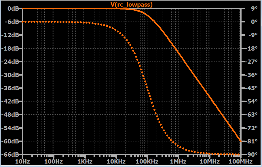
On this plot, the horizontal axis is labelled in hertz rather than rad/s. This is completely normal:

$$\omega =2\pi f$$

where $f$ is frequency in hertz and $\omega$ is angular frequency in rad/s. The underlying response is the same; only the horizontal coordinate has been expressed in different units.

---

A reliable procedure for evaluating $H(j\omega )$

When a problem gives a transfer function and asks for the response at a specified angular frequency, use the following procedure.

1. Write the transfer function exactly as given.
   Keep $s$ symbolic initially.

2. Write the requested angular frequency with units.
   For example,

   $${\omega }_0=5000\text{rad/s}$$

3. Substitute $s=j{\omega }_0$.
   This is the critical operation:

   $$H(j{\omega }_0)={H(s)|}_{s=j{\omega }_0}$$

4. Simplify the result as a complex number.
   Rectangular form, such as $a+jb$, is often useful. Polar form is useful for gain and phase.

5. State what the result means.
   It is the output-to-input phasor ratio at the selected frequency.

There are two notation errors to avoid:

$$H({\omega }_0)$$

is not generally the same thing as $H(j{\omega }_0)$, because it omits the imaginary unit. And if the problem specifies angular frequency, do not substitute $f$ directly for $\omega$. Convert using $\omega =2\pi f$ first.

---

Worked example: RC low-pass response at one frequency

Consider an RC low-pass transfer function with

$$RC=100\mu \text{s}$$

and

$$H(s)=\frac{1}{1+sRC}$$

Evaluate the response at

$${\omega }_0=5000\text{rad/s}$$

First, replace $s$ with $j{\omega }_0$:

$$H(j5000)=\frac{1}{1+j(5000)(100\times 10^{-6})}$$

The dimensionless product is

$${\omega }_{0}RC=(5000)(100\times 10^{-6})=0.5$$

Therefore,

$$H(j5000)=\frac{1}{1+j0.5}$$

To express this in rectangular form, multiply numerator and denominator by the complex conjugate $1-j0.5$:

$$H(j5000)=\frac{1-j0.5}{(1+j0.5)(1-j0.5)}$$ $$H(j5000)=\frac{1-j0.5}{1+0.5^2}$$ $$H(j5000)=0.8-j0.4$$

This is the complete frequency-response value at $5000\text{rad/s}$.

Its magnitude, included here simply to interpret the complex result, is

$$\left|H(j5000)\right|=\sqrt{0.8^2+(-0.4{)}^2}$$ $$\left|H(j5000)\right|\approx 0.894$$

So a sinusoidal input at this angular frequency produces an output whose amplitude is about $89.4\%$ of the input amplitude, with a negative phase angle. The exact calculation of that phase angle is the focus of a later lesson.

A quick limiting-behavior check supports the result. For this low-pass circuit,

$$H(j0)=1$$

so a DC input is passed unchanged. At very large $\omega$, the term $j\omega RC$ dominates the denominator, making the magnitude of $H(j\omega )$ small. The value $0.894$ at a moderate angular frequency is consistent with that gradual attenuation.

---

A second example: a transfer function with $s$ in the numerator

The method is not restricted to low-pass expressions. Suppose

$$H(s)=\frac{s+1000}{s+10000}$$

Evaluate the frequency response at

$${\omega }_0=1000\text{rad/s}$$

Substitute $s=j1000$:

$$H(j1000)=\frac{j1000+1000}{j1000+10000}$$

Factor out $1000$ from both numerator and denominator:

$$H(j1000)=\frac{1+j}{10+j}$$

Now multiply by the conjugate of the denominator:

$$H(j1000)=\frac{(1+j)(10-j)}{(10+j)(10-j)}$$ $$H(j1000)=\frac{11+j9}{101}$$ $$H(j1000)\approx 0.109+j0.089$$

Again, this is a complex ratio, not merely a real “voltage gain.” At $\omega =1000\text{rad/s}$, both amplitude scaling and phase shift are present.

The algebra may look different from one transfer function to another, but the central action never changes:

$$\boxed{H(j{\omega }_0)=H(s)\text{ with }s\text{ replaced by }j{\omega }_0}$$

---

Common conceptual traps

Confusing the function with one evaluated value

These are three different levels of description:

$$H(s)=\frac{1}{1+sRC}$$

is the transfer function.

$$H(j\omega )=\frac{1}{1+j\omega RC}$$

is the frequency response as a function of frequency.

$$H(j5000)=0.8-j0.4$$

is one response value, evaluated at one angular frequency for $RC=100\mu \text{s}$.

Writing the intermediate $H(j\omega )$ step is good engineering practice. It makes it easy to detect an incorrect substitution before numbers obscure the structure.

Substituting $s=\omega$

The substitution is not

$$s=\omega$$

but

$$s=j\omega$$

Omitting $j$ removes the phase behavior that capacitors and inductors produce. The result would no longer represent sinusoidal steady-state phasor analysis.

Mixing hertz and rad/s

If a problem gives

$$f=1\text{kHz}$$

then the required angular frequency is

$$\omega =2\pi (1000)$$ $$\omega \approx 6283\text{rad/s}$$

Only then should you substitute $s=j6283$. In contrast, if the stated value is already $1000\text{rad/s}$, no $2\pi$ conversion is needed.

Treating the denominator as a real number

For an expression such as

$$\frac{1}{1+j\omega RC}$$

the denominator is complex for every nonzero $\omega$. Do not simplify it as though it were $1+\omega RC$. Retain $j$, then use complex-number algebra when a numerical result is needed.

---

Key takeaways

The transfer function

$$H(s)=\frac{V_o(s)}{V_i(s)}$$

is the general Laplace-domain description of a circuit’s voltage ratio. The frequency response is obtained by restricting that transfer function to sinusoidal steady-state conditions:

$$H(j\omega )={H(s)|}_{s=j\omega }$$

At a specified angular frequency ${\omega }_0$, evaluate the response by substituting

$$s=j{\omega }_0$$

and simplifying the resulting complex number. That number represents the output phasor divided by the input phasor at the chosen frequency.

Next, you will separate this complex response into its magnitude, $|H(j\omega )|$, and gain in decibels—the quantities used to read and construct filter magnitude plots.