Selecting an Open-Weight Model and Quantization for a Memory Budget

A model file can appear to “fit” a machine and still fail during generation. The reason is the distinction you have already developed: weights are a mostly fixed cost, while the KV cache grows with context and active requests. On top of both sit runtime workspaces, the operating system, and other processes.

In this lesson, you will turn a raw memory budget into a defensible choice of open-weight model, format, and quantization. The goal is not to find the smallest file that launches; it is to choose the highest-quality viable option that still has room for the context length and concurrency your workload needs.

---

Start with the real memory budget

A device’s advertised memory is not your model-serving budget.

For a discrete GPU, the relevant capacity is generally GPU VRAM. System RAM may be plentiful, but moving parts of an actively used model over PCIe is usually much slower than keeping them on the GPU. For Apple Silicon, CPU, GPU, and Neural Engine share unified memory. This avoids a separate host-to-VRAM copy, but it also means macOS, browser tabs, Python processes, and the model all compete for one pool.

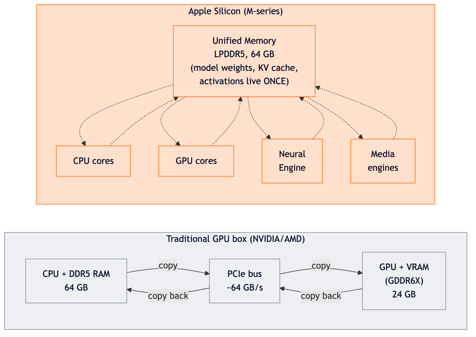
Treat the available capacity as a budgeting problem. Use the same unit throughout, preferably GiB.

$$M_{\mathrm{usable}}=M_{\mathrm{device}}-M_{\mathrm{baseline}}-M_{\mathrm{reserve}}$$

Where:

• $M_{\mathrm{device}}$ is physical VRAM or unified memory.
• $M_{\mathrm{baseline}}$ is memory already needed by the operating system and normal applications.
• $M_{\mathrm{reserve}}$ is safety headroom for transient allocations, memory fragmentation, and imperfect estimates.

A practical initial reserve is often 15–30% of device memory, adjusted after measurement. On a laptop, leave more room if other applications will remain open. A configuration that uses nearly all memory may launch successfully yet become unstable when prompts are longer, a second request arrives, or another application allocates memory.

The model configuration must satisfy:

$$M_{\mathrm{planned}}=M_{\mathrm{weights}}+M_{\mathrm{KV}}+M_{\mathrm{runtime}}\le M_{\mathrm{usable}}$$

The runtime term includes temporary compute buffers, activations, tokenizer overhead, and engine-specific allocations. It is hard to predict exactly from first principles, so selection begins with an estimate and ends with an actual load test.

---

Quantization changes the weight budget

An unquantized model stores each learned parameter at a relatively high numerical precision, commonly FP16 or BF16. Quantization represents weights with fewer bits, substantially reducing their storage and memory footprint. It also introduces approximation error, so less memory is purchased at the cost of some possible quality loss.

For a rough lower-bound estimate:

$$M_{\mathrm{weights},\mathrm{decimal}\mathrm{GB}}\approx \frac{P_{\mathrm{B}}\times b_{\mathrm{effective}}}{8}$$

Here:

• $P_{\mathrm{B}}$ is the number of parameters in billions;
• $b_{\mathrm{effective}}$ is the average stored bits per weight;
• the division by $8$ converts bits to bytes.

For an $8$B-parameter model, the idealized weight-only estimate is:

Stored precision	Approximate weight memory
FP16 / BF16	$16$ GB
8-bit	$8$ GB
6-bit	$6$ GB
4-bit	$4$ GB

These are planning estimates, not promises. A real quantized artifact contains metadata and may use mixed precision, scales, and block information. Thus, a GGUF file labelled “Q4” may average closer to $4.5$–$5$ bits per weight rather than exactly $4$.

The naming convention is helpful but not fully standardized:

• Q8 generally means roughly eight-bit weights and preserves more of the original model.
• Q4 means roughly four-bit weights and is much smaller.
• Names such as Q4_K_M, Q5_K_M, or IQ4 identify a particular quantization family and recipe, not merely a universal quality ranking.
• Two files with the same nominal bit level can differ in size, speed, and output quality because the quantization procedure differs.

Watch the following segments for a concise visual account of what the labels mean, then return to the memory-selection method below.

For local inference, do not equate file size, weight-memory estimate, and total runtime memory:

Quantity	What it answers	What it leaves out
Download size	Can I store the artifact?	KV cache and runtime allocations
Weight estimate	Can the core parameters plausibly reside in memory?	Context, concurrency, work buffers
Measured process/device memory	Does this actual engine configuration run safely?	Whether it meets quality and latency needs

A memory-mapped file may also blur the distinction between “loaded” and “resident” memory on some operating systems. For planning, use the published artifact size as useful evidence, then validate with the inference engine you will actually deploy.

---

The KV cache decides whether a model operates within budget

A selected quantization can fit in memory at startup and still be wrong for the intended workload. The common cause is allocating too little for the KV cache.

From the previous lesson, an approximate KV-cache requirement is:

$$M_{\mathrm{KV},\mathrm{bytes}}=2\times L\times n_{\mathrm{kv}}\times d_{\mathrm{head}}\times T\times B\times s$$

Where:

• $L$ is number of transformer layers;
• $n_{\mathrm{kv}}$ is the number of key-value heads;
• $d_{\mathrm{head}}$ is head dimension;
• $T$ is cached context length in tokens;
• $B$ is the number of simultaneous active sequences;
• $s$ is bytes per stored KV element.

The factor of $2$ accounts for both keys and values. The important operational consequence is that context length and active concurrency are multipliers, not cosmetic settings.

Suppose an $8$B model has:

• $32$ layers;
• $8$ KV heads;
• head dimension $128$;
• FP16 KV cache, so $s=2$ bytes;
• an $8,192$-token context;
• one active request.

Its KV-cache estimate is:

$$M_{\mathrm{KV}}=2\times 32\times 8\times 128\times 8192\times 1\times 2$$ $$M_{\mathrm{KV}}=1,073,741,824\text{bytes}\approx 1\mathrm{GiB}$$

At four active sequences with the same context target, the cache alone is approximately $4\mathrm{GiB}$. If you double the context, it doubles again.

This is why the right question is not:

“Can my machine run an 8B model?”

It is:

“Can this engine run this 8B model at this quantization, with this context limit and this active-request limit, while preserving safety headroom?”

---

Use artifact tables as evidence, not as universal truth

The llama.cpp quantization documentation provides a useful reality check: actual quantized sizes do not perfectly match the ideal $P\times b/8$ estimate. Its tables also demonstrate that quantization variants can affect speed as well as size.

Three cautions apply when reading such a table:

1. Stay model-specific. A quant size for one architecture is not a size estimate for every “8B” model. Architecture metadata and packaging differ.

2. Stay engine-specific. GGUF is designed for engines in the llama.cpp ecosystem. A Transformers deployment using bitsandbytes, an MLX model, and a GGUF model are different formats and may have different memory behavior.

3. Treat output quality as an empirical requirement. Higher bit width commonly preserves model behavior better, but quality impact depends on model family and task. A coding workflow, multilingual application, or structured-output service may reveal degradation that casual chat does not.

---

A complete selection example

Assume you have a $16\mathrm{GiB}$ Apple Silicon laptop and want a local interactive assistant for development. You want one active request, up to $8,192$ tokens of total context, and a stable process rather than a machine that swaps memory under load.

First budget the machine:

Memory item	Budget
Physical unified memory	$16\mathrm{GiB}$
macOS and normal applications	$-4\mathrm{GiB}$
Safety reserve	$-1.5\mathrm{GiB}$
Usable planned budget	$10.5\mathrm{GiB}$

Now consider a capable open-weight 8B instruct model in a GGUF format, because the next lesson will use a local engine that can run such an artifact. From the earlier KV calculation, allocate approximately $1\mathrm{GiB}$ for one $8$K request. Reserve an additional $1.5\mathrm{GiB}$ for runtime and temporary allocations.

That leaves roughly:

$$10.5-1-1.5=8\mathrm{GiB}$$

for weights.

Using the llama.cpp table as an example of realistic 8B-class GGUF artifacts:

Candidate quantization	Approximate artifact size	Planned total with $1$ GiB KV and $1.5$ GiB runtime	Selection result
F16	about $15\mathrm{GiB}$	well over budget	Reject
Q8_0	about $8\mathrm{GiB}$	around or above budget	Reject for a stable laptop baseline
Q6_K	about $6.1\mathrm{GiB}$	about $8.6\mathrm{GiB}$	Fits with useful margin
Q4_K_M	about $4.6\mathrm{GiB}$	about $7.1\mathrm{GiB}$	Fits with more margin

A defensible initial choice is therefore:

An open-weight 8B instruct model, in GGUF Q6_K when available, with an 8K context limit and one active sequence.

Why Q6_K rather than automatically choosing Q4_K_M? Both fit, but Q6 leaves enough headroom in this particular budget while retaining more weight precision. Q4_K_M becomes the better operational choice if you need longer contexts, multiple active requests, or more room for other applications. The correct choice is the highest-fidelity quantization that fits the full planned workload, not the largest quantization that barely loads.

Notice what this conclusion does not claim:

• It does not claim that every $16\mathrm{GiB}$ Mac will behave identically.
• It does not claim Q6 is universally better for every task.
• It does not promise that an $8$B model meets every quality requirement.
• It does not justify increasing concurrency beyond one request.

It is a bounded engineering decision with clear assumptions that can be benchmarked and revised.

---

A repeatable model-selection procedure

Use this procedure whenever you face a new hardware budget.

1. Write the workload contract first

Record the requirements that affect model selection:

• target task: chat, summarization, code assistance, extraction, or classification;
• required languages and specialized capabilities;
• maximum prompt plus generated-output length;
• intended active concurrency;
• latency objective;
• engine and format constraint;
• licensing and redistribution requirements.

“Open weight” means the parameters can be obtained and run, but it does not automatically mean unrestricted commercial use or redistribution. Read the model’s license and model card before treating it as deployable in a product.

2. Choose compatible candidate families

For the upcoming local Apple Silicon baseline, a practical route is an instruct-tuned open-weight model offered in a local-engine-compatible format such as GGUF for llama.cpp, or a variant explicitly supported by MLX.

Do not select a quantization first and then search for a model that happens to have that label. Select candidates that meet the task and license constraints, then compare their available formats and quants.

3. Reserve non-weight memory before comparing files

Calculate:

$$M_{\mathrm{weight}\mathrm{allowance}}=M_{\mathrm{usable}}-M_{\mathrm{KV}}-M_{\mathrm{runtime}}$$

Use intended maximum context and active sequence count, not the model card’s theoretical maximum context. A $128$K context-capable model is perfectly usable at $8$K if that is your actual requirement; allocating its full theoretical context on a constrained machine is often impractical.

4. Prefer the best-supported quant below the allowance

Within the available formats:

• start at the highest precision likely to fit;
• check actual artifact size and effective bits per weight;
• step down only when the full workload exceeds budget;
• leave deliberate headroom;
• avoid extremely low-bit variants merely to claim that a larger model runs.

For small models, aggressive quantization can damage the behavior you hoped to gain from selecting that model in the first place. A slightly smaller model at a robust quantization can be more useful than a larger one forced into a severely compressed variant.

5. Validate the selection in the real engine

A memory plan is a hypothesis. Validate it with the intended engine and settings:

• load the model;
• set the exact context limit;
• run a representative long prompt;
• generate a representative long output;
• inspect process and device memory;
• repeat with the intended number of active requests.

Record model name, source, quantization, engine version, context setting, and observed memory. This turns “it ran on my laptop” into reproducible evidence.

---

Key takeaways

• Model selection is a total-memory decision: weights, KV cache, runtime allocations, operating-system use, and safety headroom all matter.
• Quantization reduces weight memory, but nominal labels such as Q4 and Q6 are approximate families rather than universal guarantees of size or quality.
• The KV cache scales with both context length and active concurrency, so a model that loads may still fail under realistic requests.
• On Apple Silicon, unified memory eliminates a separate VRAM pool but makes careful system-wide headroom especially important.
• Select the highest-quality model and quantization that fit the full intended workload with margin, then confirm the result by measurement.
• For a constrained local baseline, an 8B-class instruct model at a moderate GGUF quantization is often a more defensible starting point than forcing a much larger model into an extreme quantization.

Next, you will put this decision into practice by serving a small quantized model on Apple Silicon with llama.cpp or MLX and querying it from Python.