Entropy Changes in Ideal Gas Processes

Hello! Welcome to our next lesson on thermodynamics.

In our last session, we established the Principle of Increasing Entropy, which provides a definitive test for whether a process is possible ($\Delta S_{\text{total}}\ge 0$). We saw that to apply this principle, we need to calculate the entropy change of the system ($\Delta S_{\text{system}}$).

Today's lesson focuses on exactly that. Our goal is to calculate entropy changes for ideal gases undergoing various thermodynamic processes. Air, the working fluid in many aerospace applications, is often modeled as an ideal gas. Mastering these calculations is therefore essential for analyzing components like compressors, turbines, and nozzles in a jet engine. We'll develop the core equations you'll use throughout the rest of this course.

1. The Foundation: T-ds Relations

To find the change in entropy, we need to relate it to other properties we can measure, like temperature, pressure, and volume. The starting points for these relationships are the two Gibbs equations, also known as the T-ds relations. For an internally reversible process, they are:

1. $Tds=du+Pdv$
2. $Tds=dh-vdP$

Here, $s$ is specific entropy, $u$ is specific internal energy, $h$ is specific enthalpy, $T$ is temperature, $P$ is pressure, and $v$ is specific volume.

For an ideal gas, we know that $du=c_{v}dT$, $dh=c_{p}dT$, and from the ideal gas law, $Pv=RT$. By substituting these into the Gibbs equations and rearranging, we can get expressions for the change in entropy, $ds$.

The following image from NASA provides a clear, step-by-step derivation of the final integrated formulas we'll be using. It's a great visual summary that aligns with your preference for formula-based approaches.

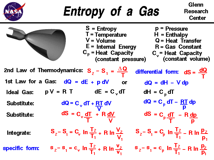
As the derivation shows, we arrive at two main equations for the change in specific entropy, $\Delta s=s_2-s_1$:

$\Delta s={\int }_1^2{c}_v(T)\frac{dT}{T}+R\ln \left(\frac{v_2}{v_1}\right)$
$\Delta s={\int }_1^2{c}_p(T)\frac{dT}{T}-R\ln \left(\frac{P_2}{P_1}\right)$

The main challenge is how to handle the integrals involving specific heats, $c_v$ and $c_p$, which are dependent on temperature. This leads to two common methods.

2. Two Methods for Calculating Entropy Change

There are two primary approaches to solving these equations, depending on the required accuracy and the magnitude of the temperature change.

Method 1: Approximate Analysis (Assuming Constant Specific Heats)

For processes where the temperature range is not too large (e.g., a few hundred Kelvin), we can simplify the calculation by assuming the specific heats $c_p$ and $c_v$ are constant. We typically use an average value for the given temperature range.

With this assumption, $c_p$ and $c_v$ come out of the integral, and $\int (1/T)dT=\ln (T_2/T_1)$. The entropy change equations become:

$\Delta s=c_{v,\text{avg}}\ln \left(\frac{T_2}{T_1}\right)+R\ln \left(\frac{v_2}{v_1}\right)$
$\Delta s=c_{p,\text{avg}}\ln \left(\frac{T_2}{T_1}\right)-R\ln \left(\frac{P_2}{P_1}\right)$

This method is computationally simpler but less accurate, especially for the large temperature changes seen in gas turbines.

Method 2: Exact Analysis (Using Variable Specific Heats)

For higher accuracy, especially in aerospace applications, we must account for the fact that specific heats change with temperature. To avoid performing the complex integral $\int (c_p(T)/T)dT$ every time, thermodynamicists have pre-calculated its value and tabulated it.

We define a new property called standard entropy, denoted as $s^o$, which is a function of temperature only:
$s^o(T)={\int }_0^T\frac{c_p(T)}{T}dT$
The value of $s^o$ at various temperatures can be found in ideal gas property tables (e.g., for air).

Using this, the entropy change is the difference in these tabulated values plus the pressure term:
$\Delta s=s^o(T_2)-s^o(T_1)-R\ln \left(\frac{P_2}{P_1}\right)$

This is the exact method because it correctly accounts for the variation of specific heat with temperature.

3. Special Case: Isentropic Processes ($\Delta s=0$)

A process that is both adiabatic (no heat transfer) and reversible (no friction or other losses) has zero entropy change. This is called an isentropic process ($\Delta s=0$). This is an important idealization for components like compressors and turbines in a jet engine.

By setting $\Delta s=0$ in our previous equations, we can derive special relationships between properties for an isentropic process.

Using Constant Specific Heats

If we set $\Delta s=0$ in the approximate formula, we get:
$0=c_p\ln \left(\frac{T_2}{T_1}\right)-R\ln \left(\frac{P_2}{P_1}\right)$
Using the relationships $R=c_p-c_v$ and $k=c_p/c_v$, this can be rearranged into the famous isentropic relations:
$\frac{T_2}{T_1}={\left(\frac{P_2}{P_1}\right)}^{(k-1)/k}\frac{T_2}{T_1}={\left(\frac{v_1}{v_2}\right)}^{k-1}\frac{P_2}{P_1}={\left(\frac{v_1}{v_2}\right)}^k$
These are powerful, quick-use formulas for analyzing ideal processes.

Using Variable Specific Heats (Exact Analysis)

For a more accurate isentropic analysis, we set $\Delta s=0$ in the exact equation:
$0=s^o(T_2)-s^o(T_1)-R\ln \left(\frac{P_2}{P_1}\right)⟹\ln \left(\frac{P_2}{P_1}\right)=\frac{s^o(T_2)-s^o(T_1)}{R}$
To make this easier to use, we define two new properties, relative pressure ($P_r$) and relative volume ($v_r$), which are also functions of temperature and are tabulated for ideal gases. They are defined such that for an isentropic process:
$\frac{P_2}{P_1}=\frac{P_{r2}}{P_{r1}}\text{and}\frac{v_2}{v_1}=\frac{v_{r2}}{v_{r1}}$
This method allows for a highly accurate analysis of isentropic processes by simply looking up values in a table, avoiding the less accurate constant specific heat assumption.

4. Putting It All Together: Worked Examples

The best way to solidify these concepts is to see them applied. The following video examples demonstrate how to solve problems using the formulas we've just discussed.

These examples show the versatility of the entropy change equations. You select the appropriate formula based on the information you have (T, P, v), and you decide whether to use the approximate or exact method based on the required accuracy.

Conclusion

In this lesson, you have learned the essential methods for calculating entropy changes in ideal gases, a critical skill for analyzing thermodynamic cycles.

Key Takeaways:

• There are two main formulas for calculating entropy change in an ideal gas, one relating (T, v) and the other relating (T, P).
• Approximate Analysis (Constant Specific Heats): A simpler method suitable for small temperature changes, using the familiar isentropic relations with the specific heat ratio $k$.
• Exact Analysis (Variable Specific Heats): A more accurate method crucial for high-temperature applications. It uses the tabulated standard entropy ($s^o$) for general processes and relative pressure ($P_r$) for isentropic processes.
• An isentropic process ($\Delta s=0$) is a key idealization for components like turbines and compressors, and we have specific, simplified relations to analyze them.

Preview of the Next Lesson:
Now that we can calculate entropy change, we are ready to analyze entire thermodynamic cycles. In the next lesson, we will analyze the Carnot cycle. The Carnot cycle represents the most efficient possible cycle that can operate between two temperature reservoirs, serving as the ultimate benchmark against which all real heat engines, including jet engines, are measured.