Op-Amp Integrator & Differentiator

Hello! Welcome back to our course on Radioelectronics.

Introduction

Approximate time to complete: 1 hour

In our last lesson, we saw how op-amps can be configured to perform arithmetic operations like addition, subtraction, and scaling, creating summing and difference amplifiers. We learned that these circuits are the foundation of analog signal processing.

Today, we'll take this a step further by introducing capacitors into our op-amp circuits. This simple change allows us to build circuits that perform calculus operations. The learning outcome for this lesson is to understand and analyze Op-Amp Integrator and Differentiator Circuits. We will explore how these circuits work, their practical limitations, and how they are used for wave-shaping.

Recap from previous lessons:

Op-Amp Golden Rules (with negative feedback):
1. No current flows into the input terminals ( $I_{+} = I_{-} = 0$ ).
2. The voltage at the input terminals is the same ( $V_{+} = V_{-}$ ), which often creates a virtual ground at the inverting input if the non-inverting input is grounded.
Capacitor Current-Voltage Relationship: The current through a capacitor is proportional to the rate of change of the voltage across it: $I_{C} = C \frac{d V _{C}}{d t}$ . This relationship is the key to today's lesson.

Let's begin with the integrator.

The Op-Amp Integrator

The integrator circuit produces an output voltage that is proportional to the integral of the input voltage over time. We can create this circuit by modifying the standard inverting amplifier: we simply replace the feedback resistor with a capacitor.

1. Derivation and Ideal Operation

To understand how this circuit works, let's derive its input-output relationship. The video below provides an excellent step-by-step derivation.

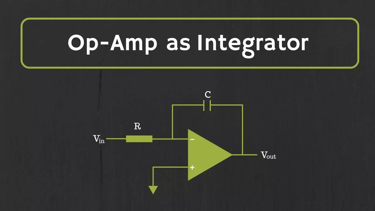
Please watch the first section of this video from ALL ABOUT ELECTRONICS (00:48 - 04:22). It clearly explains the derivation using the principles we've already covered.

Let's summarize the derivation you just saw.

We start with the inverting configuration. The non-inverting input is grounded, so the inverting input is at a virtual ground ( $V_{-} = 0$ ).
We apply Kirchhoff's Current Law (KCL) at the inverting node. The input current $I_{in}$ flowing through resistor $R$ must be equal to the current $I_{C}$ flowing through the feedback capacitor $C_{f}$ , since no current enters the op-amp.
$I_{in} = I_{C}$
We express these currents using Ohm's Law and the capacitor's V-I relationship:
$\frac{V _{in} - 0}{R} = C_{f} \frac{d ( V _{-} - V _{o u t} )}{d t}$
Since $V_{-} = 0$ , this simplifies to:
$\frac{V _{in}}{R} = C_{f} \frac{d ( - V _{o u t} )}{d t} = - C_{f} \frac{d V _{o u t}}{d t}$
Rearranging and integrating both sides with respect to time gives us the final equation for the ideal integrator:
$\int d V_{o u t} = \int - \frac{1}{R C _{f}} V_{in} (t) d t$
$V_{o u t} (t) = - \frac{1}{R C _{f}} \int_{0}^{t} V_{in} (τ) d τ + V_{o u t} (0)$
where $V_{o u t} (0)$ is the initial voltage across the capacitor at $t = 0$ .

2. Wave-Shaping Applications

The mathematical relationship above leads to some powerful wave-shaping capabilities.

Please continue watching the video from 04:22 to 05:37 to see how the integrator responds to different input waveforms.

As you saw, the integrator performs the following transformations:

Square Wave Input → Triangular Wave Output: Integrating the constant positive/negative levels of a square wave produces linearly increasing/decreasing ramps.
Sinusoidal Input → Cosinusoidal Output: Integrating $sin (ω t)$ yields $- cos (ω t)$ , resulting in a 90-degree phase shift.
DC Step Input → Ramp Output: Integrating a constant DC voltage produces a ramp function whose slope is determined by the input voltage and the $RC$ time constant.

3. Practical Limitations and Solutions

The ideal integrator circuit has a major flaw that makes it unusable in practice. At DC ( $f = 0$ ), a capacitor's impedance ( $X_{C} = 1/ (jω C)$ ) is infinite. This means the feedback loop is open for DC signals, and the op-amp's gain becomes its massive open-loop gain.

This leads to two critical problems:

Any small DC offset voltage at the input (which is always present in real op-amps) gets amplified by this huge gain.
The output voltage quickly drifts and slams into the op-amp's positive or negative supply rail (saturation).

Watch the next segment of the video (05:37 - 09:49) to understand these limitations and the simple, elegant solution.

The solution is to add a large feedback resistor, $R_{f}$ , in parallel with the feedback capacitor $C_{f}$ . This is called a practical integrator.

At DC/Low Frequencies: The capacitor acts as an open circuit, but now $R_{f}$ provides the feedback path. The circuit behaves like a simple inverting amplifier with a finite gain of $- R_{f} / R$ . This prevents saturation by limiting the DC gain.
At High Frequencies: The capacitor's impedance becomes very low, effectively shorting out the parallel resistor $R_{f}$ . In this range, the circuit behaves like the ideal integrator.

4. Frequency Response and Design

The practical integrator is effectively an active low-pass filter.

Watch the final segment on frequency response (09:49 - 12:12).

Here are the key takeaways for design:

The circuit has a cutoff frequency $f_{L} = \frac{1}{2 π R _{f} C _{f}}$ .
For frequencies below $f_{L}$ , the circuit acts as an inverting amplifier with a constant gain of $- R_{f} / R$ .
For frequencies above $f_{L}$ , the gain starts to roll off at -20 dB/decade, and the circuit behaves as an integrator.
Rule of Thumb: For proper integration, the input signal's frequency $f_{in}$ should be at least 10 times higher than the cutoff frequency $f_{L}$ .

The Op-Amp Differentiator

As you might guess, if replacing a resistor with a capacitor creates an integrator, swapping their positions should do the opposite. The differentiator circuit produces an output proportional to the time derivative of the input signal.

1. Derivation and Ideal Operation

The ideal differentiator is an inverting amplifier with the input resistor replaced by a capacitor.

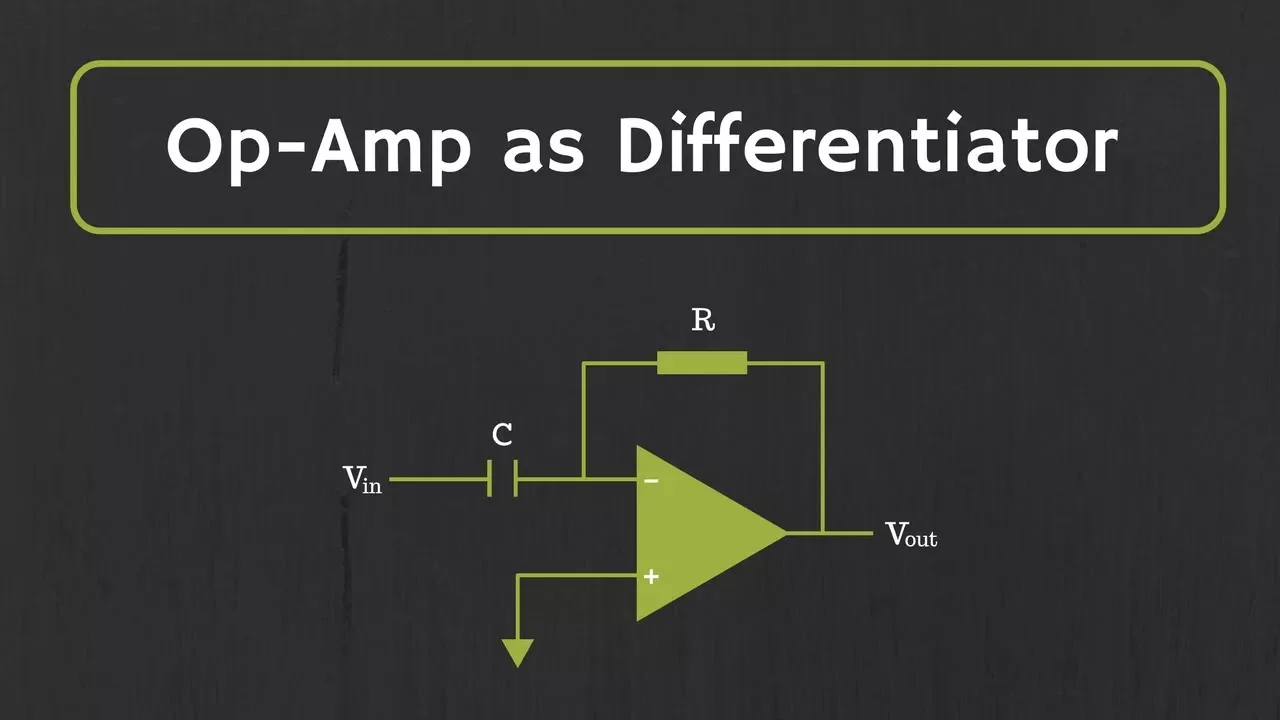
Please watch the derivation in this video from ALL ABOUT ELECTRONICS (01:39 - 03:39).

The derivation is analogous to the integrator's:

KCL at the virtual ground node: $I_{C} = I_{f}$ .
Express the currents:
$C \frac{d ( V _{in} - V _{-} )}{d t} = \frac{V _{-} - V _{o u t}}{R _{f}}$
With $V_{-} = 0$ , this simplifies to:
$C \frac{d V _{in}}{d t} = - \frac{V _{o u t}}{R _{f}}$
Solving for $V_{o u t}$ gives the ideal differentiator equation:
$V_{o u t} (t) = - R_{f} C \frac{d V _{in} ( t )}{d t}$

2. Wave-Shaping Applications

Watch the next short segment (03:39 - 04:26) to see how it transforms common waveforms.

Key transformations include:

Triangular Wave Input → Square Wave Output: The constant positive/negative slopes of a triangular wave result in constant positive/negative output voltages.
Square Wave Input → Spike Output: The theoretically infinite slope at the edges of a square wave produces sharp voltage spikes (impulses).
Sinusoidal Input → Cosinusoidal Output: Differentiating $sin (ω t)$ yields $cos (ω t)$ .

3. Practical Limitations and Solutions

The ideal differentiator has the opposite problem of the integrator: it's a high-pass filter. Its gain, $∣ A ∣ = ω R_{f} C$ , increases linearly with frequency.

This leads to severe practical issues. Watch the segment on limitations from 04:26 to 07:47.

The key problems are:

High-Frequency Noise Amplification: Any high-frequency noise present on the input signal will be amplified much more than the desired signal, often dominating the output.
Instability: The rising gain with frequency can cause the circuit to become unstable and oscillate.
Low Input Impedance: At high frequencies, the capacitor's impedance becomes very low, which can heavily load the circuit providing the input signal.

Now, watch the section on the practical differentiator design (07:47 - 09:56).

The fixes involve adding two components:

A small resistor $R_{i}$ in series with the input capacitor $C$ : This limits the high-frequency gain to a finite value ( $- R_{f} / R_{i}$ ) and ensures a minimum input impedance of $R_{i}$ at high frequencies.
A small capacitor $C_{f}$ in parallel with the feedback resistor $R_{f}$ : This adds a second pole that rolls off the gain at very high frequencies, further improving stability and noise rejection.

4. Frequency Response and Design

The practical differentiator's frequency response is more complex. It only acts as a true differentiator over a specific frequency band.

Please watch the final segment on frequency response (09:56 - 11:45).

The circuit has a frequency range where its gain increases with frequency at +20 dB/decade. This is the region of differentiation.
The series input resistor $R_{i}$ and capacitor $C$ introduce a zero that causes the gain to flatten out at a frequency $f_{1} = \frac{1}{2 π R _{i} C}$ .
Rule of Thumb: For accurate differentiation, the input signal's frequency $f_{in}$ must be significantly lower than this cutoff frequency $f_{1}$ (e.g., $f_{in} < f_{1} /10$ ).

Conclusion

In this lesson, we have seen how the simple addition of capacitors transforms our op-amp circuits into powerful tools for analog computation, capable of performing calculus.

Key Takeaways:

Op-Amp Integrator: Uses a capacitor in the feedback path to produce an output proportional to the integral of the input. Practical designs require a parallel feedback resistor to limit DC gain and ensure stability. This circuit functions as an active low-pass filter.
Op-Amp Differentiator: Uses a capacitor in the input path to produce an output proportional to the derivative of the input. Practical designs require a series input resistor and a parallel feedback capacitor to limit high-frequency gain, reduce noise, and ensure stability. This circuit functions as an active high-pass/band-pass filter.
These circuits are fundamental building blocks for creating filters and shaping waveforms, such as converting a square wave into a triangular wave and vice-versa.

In the next lesson, we will step back to formalize our understanding of the principle that has been at the heart of all these op-amp circuits: feedback. We will explore "Feedback Concepts: Positive and Negative Feedback in Amplifiers" and discover how changing the feedback type can lead to entirely new circuit behaviors.