Summing & Difference Amplifiers

Hello! Welcome back to your course on Radioelectronics.

Introduction

Approximate time to complete: 1 hour

In our previous lesson, we analyzed the fundamental inverting and non-inverting op-amp configurations. We saw how negative feedback allows us to control the op-amp's immense gain using simple resistor ratios.

Today, we will build directly on those concepts to create circuits that perform mathematical operations. The learning outcome for this lesson is to understand Summing and Difference Amplifiers. We'll explore how to configure op-amps to add multiple signals together and how to amplify only the difference between two signals. These circuits are the essential building blocks for analog signal processing and computation.

Recap from the previous lesson:

Inverting Amplifier: Output is $V_{o u t} = - \frac{R _{F}}{R _{i}} V_{in}$ . A key feature is the virtual ground at the inverting terminal.
Non-Inverting Amplifier: Output is $V_{o u t} = (1 + \frac{R _{F}}{R _{G}}) V_{in}$ . A key feature is its extremely high input impedance.
Golden Rules (with negative feedback):
1. No current flows into the input terminals ( $I_{+} = I_{-} = 0$ ).
2. The input terminals are at the same voltage ( $V_{+} = V_{-}$ ).

The Summing Amplifier

A summing amplifier does exactly what its name implies: it produces an output voltage that is a combination of its multiple input voltages. We can create both inverting and non-inverting versions.

1. The Inverting Summing Amplifier

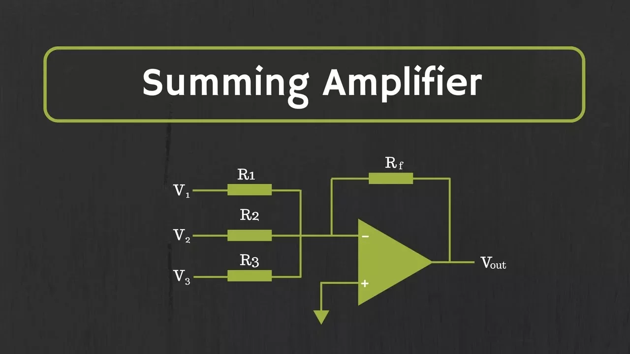
This is the most common and practical summing configuration. It's a simple extension of the inverting amplifier we studied previously, but with multiple input paths.

Please watch the first part of this video from w2aew (00:30 - 06:06). It provides an excellent explanation of the theory using the superposition principle and shows a practical demonstration on a breadboard.

Let's break down the analysis. As an engineer, you know there are often multiple valid ways to analyze a linear circuit.

Method 1: Applying KCL at the Virtual Ground

This method is a direct extension of how we analyzed the basic inverting amplifier.

Because the non-inverting input (+) is grounded, the virtual ground concept holds: $V_{-} = 0$ .
According to our golden rules, no current enters the op-amp's inverting terminal. Therefore, by KCL, the sum of the currents from the input sources must equal the current flowing away through the feedback resistor, $R_{F}$ .
$I_{1} + I_{2} + I_{3} = - I_{F}$
Using Ohm's Law and the fact that $V_{-} = 0$ :
$\frac{V _{1} - 0}{R _{1}} + \frac{V _{2} - 0}{R _{2}} + \frac{V _{3} - 0}{R _{3}} = - \frac{V _{o u t} - 0}{R _{F}}$
Solving for $V_{o u t}$ gives us the classic summing amplifier equation:
$V_{o u t} = - R_{F} (\frac{V _{1}}{R _{1}} + \frac{V _{2}}{R _{2}} + \frac{V _{3}}{R _{3}})$
$V_{o u t} = - (\frac{R _{F}}{R _{1}} V_{1} + \frac{R _{F}}{R _{2}} V_{2} + \frac{R _{F}}{R _{3}} V_{3})$

This shows that the output is the inverted, weighted sum of the inputs. The "weight" of each input is controlled by the ratio of the feedback resistor to its corresponding input resistor.

Key Advantages:

Scaling and Averaging: If we set all input resistors equal ( $R_{1} = R_{2} = R_{3} = R$ ), the circuit becomes a simple adder: $V_{o u t} = - \frac{R _{F}}{R} (V_{1} + V_{2} + V_{3})$ . If we further set $\frac{R _{F}}{R} = \frac{1}{N}$ (where N is the number of inputs), the circuit becomes an averager.
Input Isolation: Because the summing node ( $V_{-}$ ) is a virtual ground, each input source sees its input resistor connected to ground. This means the input signals do not interfere with each other, which is a significant practical advantage.

For a more detailed derivation using this KCL method and a discussion on applications like averaging and digital-to-analog conversion, this second video is a great supplement.

Focus on the segments from 00:59 to 09:24.

2. The Non-Inverting Summing Amplifier

We can also sum signals at the non-inverting input. However, the analysis is less straightforward and the circuit has some practical drawbacks.

Now, watch the next segment of the video (06:06 - 10:55). It explains the theory and shows the practical result.

The analysis here is a two-step process:

Find the voltage at the non-inverting terminal, $V_{+}$ . The inputs and their resistors form a voltage divider network. Using superposition (as explained in the video), we find the combined voltage at this node.
Amplify $V_{+}$ with a standard non-inverting gain. The rest of the circuit is a simple non-inverting amplifier with a gain of $A = 1 + \frac{R _{F}}{R _{N}}$ .

The final equation is more complex than the inverting case. For two inputs, it is:
$V_{o u t} = (1 + \frac{R _{F}}{R _{N}}) (\frac{R _{2}}{R _{1} + R _{2}} V_{1} + \frac{R _{1}}{R _{1} + R _{2}} V_{2})$

Key Disadvantage:

Input Cross-talk: Unlike the inverting summer, the voltage at the summing node ( $V_{+}$ ) changes based on all input signals. This means the inputs are not isolated from each other, which can be problematic in many designs. For this reason, the inverting summer is almost always preferred.

The Difference Amplifier

What if we want to amplify only the difference between two signals? This is a fundamental requirement in instrumentation and noise-canceling systems. The difference (or differential) amplifier achieves this by applying signals to both the inverting and non-inverting inputs simultaneously.

The provided resources do not cover this circuit, so I will guide you through its analysis myself.

The most intuitive way to analyze this circuit is with the superposition theorem.

Step 1: Analyze the contribution from $V_{1}$ (Set $V_{2} = 0$ )

When $V_{2}$ is grounded, the non-inverting terminal (+) is also held at ground potential via the resistor $R_{G}$ .
The circuit becomes a standard inverting amplifier with $V_{1}$ as its input.
The output due to $V_{1}$ is:
$V_{o u t 1} = - \frac{R _{F}}{R _{1}} V_{1}$

Step 2: Analyze the contribution from $V_{2}$ (Set $V_{1} = 0$ )

When $V_{1}$ is grounded, the circuit becomes a non-inverting amplifier.
The voltage at the non-inverting terminal, $V_{+}$ , is determined by the voltage divider formed by $R_{2}$ and $R_{G}$ :
$V_{+} = V_{2} (\frac{R _{G}}{R _{2} + R _{G}})$
The non-inverting amplifier gain is $A = 1 + \frac{R _{F}}{R _{1}}$ .
The output due to $V_{2}$ is:
$V_{o u t 2} = (1 + \frac{R _{F}}{R _{1}}) V_{+} = (1 + \frac{R _{F}}{R _{1}}) (\frac{R _{G}}{R _{2} + R _{G}}) V_{2}$

Step 3: Combine the results
The total output is the sum of the two contributions:
$V_{o u t} = V_{o u t 1} + V_{o u t 2} = (1 + \frac{R _{F}}{R _{1}}) (\frac{R _{G}}{R _{2} + R _{G}}) V_{2} - (\frac{R _{F}}{R _{1}}) V_{1}$

This expression looks complicated, but a powerful simplification occurs when the resistor ratios are balanced.

The Balanced Difference Amplifier

Let's set the resistor ratios to be equal:
$\frac{R _{2}}{R _{G}} = \frac{R _{1}}{R _{F}}$
This is the standard design practice. Let's see what happens to the term multiplying $V_{2}$ :
$(1 + \frac{R _{F}}{R _{1}}) (\frac{R _{G}}{R _{2} + R _{G}}) = (\frac{R _{1} + R _{F}}{R _{1}}) (\frac{R _{G}}{R _{2} + R _{G}})$
Divide the second fraction's numerator and denominator by $R_{G}$ :
$= (\frac{R _{1} + R _{F}}{R _{1}}) (\frac{1}{\frac{R _{2}}{R _{G}} + 1})$
Substitute our balanced condition $\frac{R _{2}}{R _{G}} = \frac{R _{1}}{R _{F}}$ :
$= (\frac{R _{1} + R _{F}}{R _{1}}) (\frac{1}{\frac{R _{1}}{R _{F}} + 1}) = (\frac{R _{1} + R _{F}}{R _{1}}) (\frac{1}{\frac{R _{1} + R _{F}}{R _{F}}}) = (\frac{R _{1} + R _{F}}{R _{1}}) (\frac{R _{F}}{R _{1} + R _{F}}) = \frac{R _{F}}{R _{1}}$
The entire complex term simplifies beautifully!

Substituting this back into our full equation for $V_{o u t}$ , we get the classic result for a balanced difference amplifier:
$V_{o u t} = \frac{R _{F}}{R _{1}} V_{2} - \frac{R _{F}}{R _{1}} V_{1}$
$V_{o u t} = \frac{R _{F}}{R _{1}} (V_{2} - V_{1})$

The output is simply the differential gain ( $\frac{R _{F}}{R _{1}}$ ) multiplied by the difference between the two input voltages. This circuit rejects any voltage that is common to both inputs (common-mode voltage), a property called Common-Mode Rejection, which is critical for extracting small signals from noisy environments.

Conclusion

In this lesson, we leveraged the fundamental principles of inverting and non-inverting amplifiers to build circuits capable of analog computation.

Key Takeaways:

Inverting Summing Amplifier: Produces an inverted, weighted sum of its inputs: $V_{o u t} = - (\frac{R _{F}}{R _{1}} V_{1} + \frac{R _{F}}{R _{2}} V_{2} + ...)$ . It is the preferred summing configuration due to excellent input isolation.
Non-Inverting Summing Amplifier: Also adds inputs, but the analysis is more complex and it suffers from input cross-talk.
Difference Amplifier: Amplifies the voltage difference between two inputs. In a balanced configuration, $V_{o u t} = \frac{R _{F}}{R _{1}} (V_{2} - V_{1})$ , allowing it to reject common-mode noise.

These "mathematical" circuits are not just theoretical curiosities; they are the workhorses behind audio mixers, sensor signal conditioning, and analog-to-digital converters.

In our next lesson, "Op-Amp Applications: Integrator and Differentiator Circuits," we will continue this theme by replacing resistors with capacitors to create circuits that perform calculus, opening the door to wave-shaping and filtering applications.