Optimizing Inference with torch.compile

Introduction

In our last lesson, we explored operator fusion as a key strategy to address the memory-bound nature of the LLM decode stage. We saw how fusing operations—either manually through packed projections or automatically with a compiler—reduces both kernel launch overhead and costly data trips to and from HBM.

Today, we're diving deep into the primary tool for automatic optimization in modern PyTorch: torch.compile. Your goal for this lesson is to go beyond simply applying it. You will learn to use torch.compile effectively and, more importantly, to measure and verify its impact on inference latency and the underlying GPU kernel execution. This process of applying an optimization and then using profiling tools to confirm its effect is a fundamental workflow for any systems engineer aiming to extract maximum performance from their hardware.

How torch.compile Works

At its core, torch.compile is a just-in-time (JIT) compiler that transforms your eager-mode PyTorch code into an optimized, lower-level representation. It's not a single monolithic block but a stack of components working in concert. Given your background in computer science, you'll recognize the classic compiler architecture.

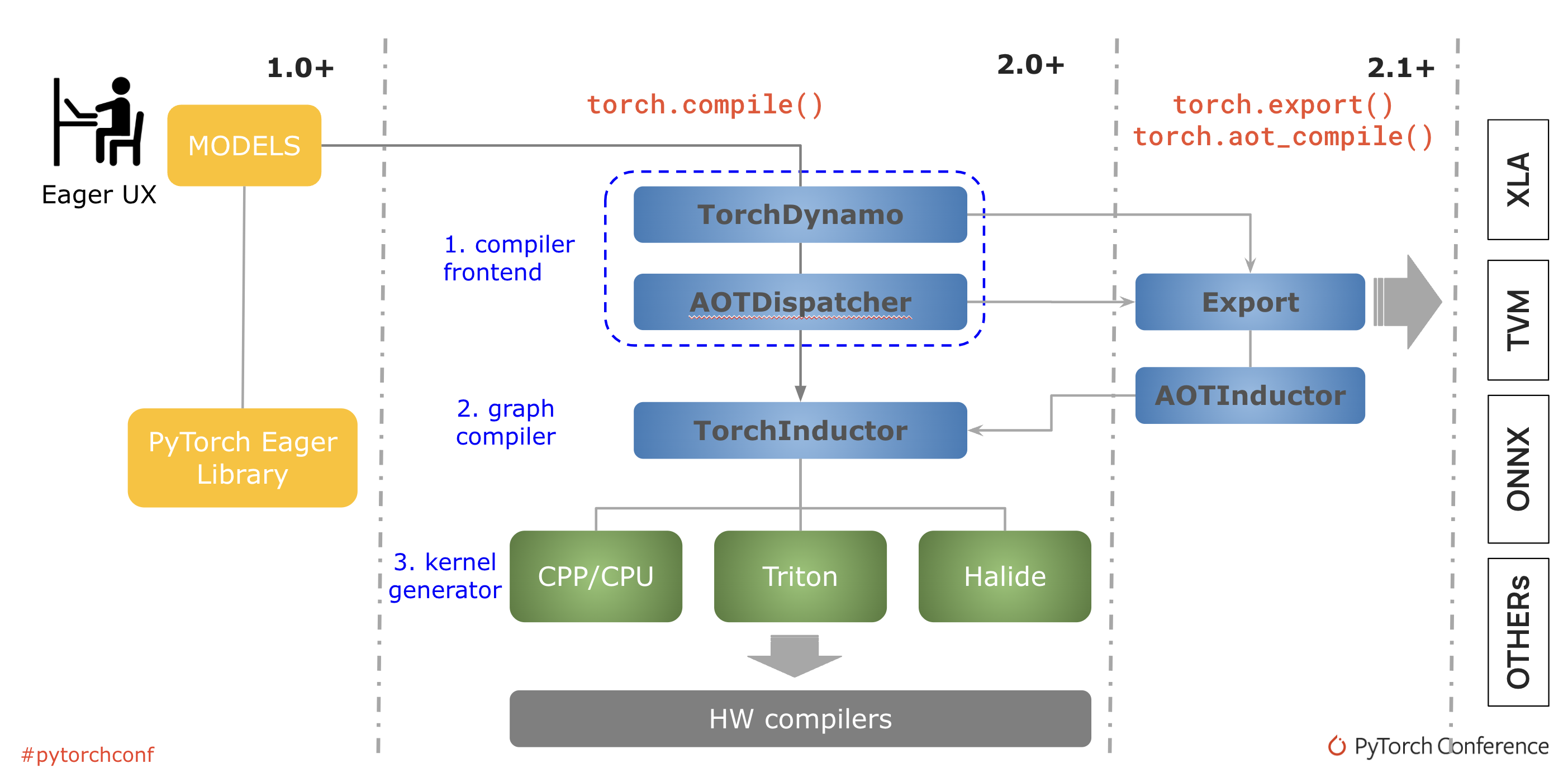
The key stages are:

1. Graph Acquisition (Frontend): TorchDynamo inspects the Python bytecode of your model's forward method during its first execution. It captures sequences of PyTorch operations into a graph. When it encounters Python features it can't safely trace (like complex control flow or certain third-party library calls), it performs a graph break, executing that part in standard eager mode before attempting to capture the next segment.
2. Graph Lowering (Backend): The captured graph is then handed off to a backend. The default and most advanced backend is TorchInductor.
3. Code Generation: TorchInductor takes the high-level graph and applies optimizations. It performs the operator fusion we discussed previously, rearranging memory layouts, and then generates highly optimized C++ or Triton kernels. These kernels are what ultimately run on the GPU.

This process has a one-time cost during the first run (the "warm-up"), but subsequent runs execute the highly optimized compiled code, often resulting in significant speedups.

From Naive PyTorch to "Blazingly Fast"

The performance difference between a naive PyTorch implementation and a compiled one can be dramatic, especially for the latency-sensitive autoregressive decoding phase of LLMs.

To see a practical demonstration of this, let's watch a presentation by Horace He, a key developer on the PyTorch team, as he introduces GPT-Fast, a minimal repository for high-performance LLM inference.

As the video demonstrates, torch.compile isn't just about fusing a few ops. It fundamentally changes the interaction between the CPU and GPU by reducing the number of individual commands, allowing the GPU to stay saturated with meaningful work.

Applying and Tuning torch.compile

Using torch.compile is straightforward. You simply wrap your model with it.

import torch




# Assume 'model' is your nn.Module instance
model = torch.compile(model)




# Now, use the compiled model as usual
# The first run will be slow due to compilation
output = model(input_tensor) 

However, torch.compile has several modes that offer trade-offs between compilation time and runtime speed.

For LLM inference, where latency is critical and the compilation cost is a one-time setup fee, mode="reduce-overhead" or mode="max-autotune" are often the best choices. They direct the compiler to prioritize minimizing CPU overhead and generating the fastest possible kernels, respectively.

Measuring the Effect: Profiling with torch.profiler

Now for the crucial part: how do we verify what the compiler did? Simply measuring wall-clock time shows that it got faster, but profiling shows why. The torch.profiler is the standard tool for this. It can capture CPU and GPU activity and generate a timeline trace that you can inspect visually.

Let's walk through the official PyTorch guide on this topic. It contains the exact code patterns and analysis techniques you'll need.

Practical Profiling Exercise

Now, let's put this into practice.

1. Take a simple transformer model (e.g., the one from our scratch implementation, or a small transformers model).
2. Write a script using the pattern from the documentation to profile a single forward pass.
3. Run 1 (Baseline): Profile the model without torch.compile. Export the Chrome trace as trace_eager.json.
4. Run 2 (Compiled): Add model = torch.compile(model, mode="reduce-overhead") after instantiating your model. Profile it again, exporting the trace as trace_compiled.json.
5. Open both traces in Chrome (chrome://tracing) and compare them.

You should observe the following differences:

• Eager Trace: The GPU timeline will show many small, distinct kernels (e.g., aten::mul, aten::add, aten::linear). You will likely see visible gaps between them, representing the launch overhead discussed in the documentation.
• Compiled Trace: The CPU timeline will show a single large CompiledFunction block. The GPU timeline will have far fewer, but much wider, kernels. These are the fused kernels generated by Inductor, often with names starting with triton_. The gaps between kernels should be significantly smaller.

This visual evidence is the most direct way to "measure the effect on GPU kernel execution." The reduction in the number of kernels and the change in their nature (from many aten ops to a few triton ops) is the physical manifestation of torch.compile's optimization work.

To see an expert walk through this exact analysis, the following video is invaluable.

Conclusion

In this lesson, we demystified torch.compile, moving it from a "magic black box" to a understandable and verifiable engineering tool. You now possess the complete workflow for applying and analyzing a major performance optimization.

Key Takeaways:

• torch.compile uses a frontend (TorchDynamo) to capture your model's computation graph and a backend (TorchInductor) to perform optimizations like operator fusion and generate efficient Triton kernels.
• It's applied with a single line of code, but different modes (default, reduce-overhead, max-autotune) allow you to trade compilation time for runtime performance.
• The primary tool to measure the effect of torch.compile is torch.profiler.
• By comparing profiler traces before and after compilation, you can visually confirm that torch.compile is working by observing a shift from many small aten kernels to a few large, fused triton kernels.
• Profiler traces are also essential for diagnosing issues, such as excessive graph breaks, which limit the compiler's effectiveness.

Preview of the Next Lesson:

While torch.profiler is excellent for a high-level view, what if you need to understand the performance of a single generated kernel? Or what if you suspect a bottleneck within a fused kernel? To answer these questions, we need to go deeper. In the next lesson, we will introduce Nsight Systems, NVIDIA's professional-grade profiler, to pinpoint compute bottlenecks at the individual CUDA kernel level and get the most detailed view possible of your GPU's activity.