Optimizing QKV Projection with Operator Fusion

Introduction

In our previous lesson, we established how to use the Roofline model to diagnose performance bottlenecks. We saw that while the prefill stage of LLM inference can be compute-bound, the token-by-token decode stage is almost always memory-bound. This means the GPU spends more time waiting for data to be moved from its main memory (HBM) than it does performing calculations.

Today, we move from diagnosis to treatment. We will implement one of the most fundamental compute optimizations for LLMs: operator fusion. You will learn to combine multiple, sequential GPU operations into a single, more efficient kernel. This technique directly addresses the memory-bound nature of many transformer operations by reducing both kernel launch overhead and data traffic to and from HBM.

At a high level, operator fusion targets inefficiencies like the one shown in the profiler trace below.

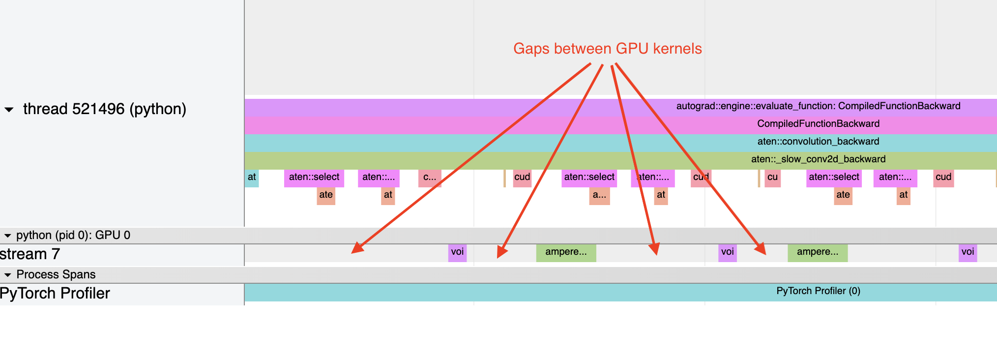
By the end of this lesson, you will have implemented fusion for the QKV projection within a transformer's attention block and understood the trade-offs between manual fusion and automatic compiler-based approaches.

The "Why" of Operator Fusion

Operator fusion improves performance in two primary ways:

1. Reduces Kernel Launch Overhead: Every time the CPU instructs the GPU to run a new kernel, there's a small but non-trivial overhead. For a sequence of small, fast operations (typical in the decode stage), this overhead can accumulate and become a significant portion of the total execution time. Fusing N kernels into one reduces this overhead by a factor of N.

2. Improves Memory Access Patterns: This is the more critical benefit for memory-bound operations. Consider a sequence of two operations, y = op1(x) and z = op2(y). Without fusion, the data flow is:

   • Read x from HBM into on-chip SRAM.
   • Compute y.
   • Write y back to HBM.
   • Read y from HBM into SRAM.
   • Compute z.
   • Write z back to HBM.

   With fusion, the intermediate write/read to HBM is eliminated:

   • Read x from HBM into SRAM.
   • Compute y and keep it in SRAM.
   • Compute z.
   • Write z back to HBM.

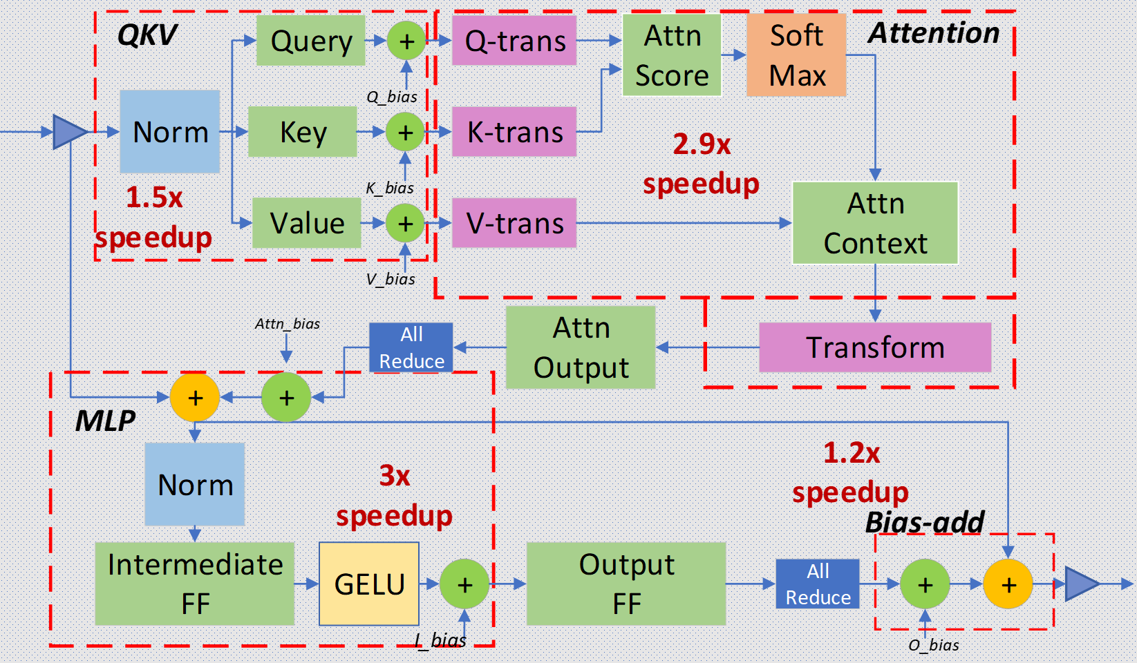
This reduction in data traffic to the "slow" main memory effectively increases the operation's arithmetic intensity (FLOPs/Byte), pushing it up and to the right on the roofline plot and closer to the compute roof. The diagram below illustrates common fusion opportunities in a transformer block.

Case Study: Fusing the QKV Projection

Let's make this concrete by focusing on the input projection in a multi-head attention block. In self-attention, the input tensor x is projected into query (Q), key (K), and value (V) tensors. A naive implementation would use three separate linear layers.

# A non-fused approach
q_proj = nn.Linear(d_model, d_model)
k_proj = nn.Linear(d_model, d_model)
v_proj = nn.Linear(d_model, d_model)

Q = q_proj(x)
K = k_proj(x)
V = v_proj(x)

This code is clean, but it launches three separate matrix multiplication (GEMM) kernels. To see a practical demonstration of this inefficiency, let's look at how a similar pattern is analyzed in a Stanford lecture on high-performance code.

Implementing Fusion: Packed Projections

The most direct way to implement QKV fusion in PyTorch is using the packed projection technique. Instead of three separate nn.Linear(d_model, d_model) layers, we use a single, wider linear layer nn.Linear(d_model, 3 * d_model) and then split the result.

# A fused approach
packed_proj = nn.Linear(d_model, 3 * d_model)

QKV_packed = packed_proj(x)
Q, K, V = torch.chunk(QKV_packed, 3, dim=-1)

This approach executes the three matrix multiplications within a single, larger GEMM kernel, significantly reducing overhead and memory traffic.

Let's study a formal implementation and its performance benefits.

As the tutorial demonstrates, this simple change can yield a noticeable speedup even on powerful hardware, especially when the operations are memory-bound. This same principle is used in other parts of the transformer, like the SwiGLU activation in the FFN layers of models like Llama.

Automatic Fusion with torch.compile

While manual packing is effective and important to understand, you often don't need to write it yourself. Modern JIT (Just-In-Time) compilers are designed to recognize these patterns and perform fusion automatically. In PyTorch, the primary tool for this is torch.compile().

When you wrap a model or module with torch.compile(), it:

1. Captures the graph of operations.
2. Passes this graph to a backend compiler (like Triton).
3. The backend analyzes the graph, fuses compatible sequential operations into single kernels, and generates highly optimized code.

Let's see how torch.compile handles the GLU example from the Stanford video.

This demonstrates the power of modern compilers. For many common fusion opportunities like QKV projection or activation functions, torch.compile is the most effective and maintainable solution.

When to Go Deeper: Custom Kernels

So if torch.compile is so effective, why would you ever write a custom kernel?

1. Novel Operations: If you are designing a new architecture with a complex operation that the compiler doesn't know how to fuse, a custom kernel might be necessary.
2. Advanced Algorithmic Changes: Compilers are excellent at fusing operations but are not (yet) capable of making high-level algorithmic changes. The classic example is FlashAttention, which is not just a fusion of existing operations but a fundamental rewrite of the attention algorithm to be IO-aware.
3. Pushing the Limits: To extract the absolute maximum performance from a specific piece of hardware, a hand-tuned kernel may outperform a compiler-generated one.

When engineers write custom kernels today, they often use Triton, a Python-based domain-specific language that simplifies GPU programming compared to lower-level CUDA C++. In fact, Triton is what torch.compile uses under the hood. For context on this decision-making process, the following discussion is insightful.

Conclusion

In this lesson, you have learned how operator fusion serves as a primary treatment for the memory-bound bottlenecks we previously diagnosed with the Roofline model.

Key Takeaways:

• Operator fusion combines multiple GPU kernels into one, reducing kernel launch overhead and, more importantly, minimizing data traffic between on-chip SRAM and off-chip HBM.
• This reduction in data movement increases an operation's arithmetic intensity, improving performance for memory-bound workloads.
• The QKV projection is a canonical example where three separate nn.Linear layers can be fused into one wider layer, a technique known as packed projection.
• torch.compile() is a powerful tool that can automatically perform fusion for many common patterns, often making it the preferred approach.
• For novel or highly complex optimizations that go beyond simple fusion (like FlashAttention), engineers write custom kernels using tools like Triton.

Preview of the Next Lesson:

We have now seen how to manually and automatically fuse operators. In the next lesson, we will apply torch.compile to our entire model and dive deep into profiling its output. You will learn to use NVIDIA's Nsight Systems, a professional-grade profiler, to inspect the CUDA kernels generated by the compiler, measure their execution time precisely, and identify any remaining bottlenecks at the hardware level.