CUDA Kernel Bottleneck Analysis with Nsight Systems

Introduction

In our last lesson, we saw how torch.compile can dramatically improve performance by fusing operations and generating optimized Triton kernels. We used torch.profiler to verify this, observing a shift from many small, distinct aten kernels to a few large, fused ones. This confirmed that an optimization occurred.

However, torch.profiler and its Chrome trace view stop at the kernel boundary. They tell you which kernels ran and for how long, but they don't tell you how efficiently those kernels used the GPU's resources. Was the fused kernel compute-bound or memory-bound? Was it stalled waiting for data? Did it suffer from inefficient memory access patterns?

To answer these questions, we need to move beyond PyTorch-level profilers and use tools that operate at the CUDA driver level. This lesson introduces NVIDIA's Nsight suite, the professional standard for GPU profiling. Your objective is to learn how to use Nsight Systems to get a system-wide overview and then use Nsight Compute to perform a deep-dive analysis of individual kernels, allowing you to pinpoint the precise reasons for performance bottlenecks.

The Profiler's Toolkit: Nsight Systems vs. Nsight Compute

NVIDIA provides two primary profiling tools, and it's crucial to understand their distinct roles. They are designed to be used together in a top-down analysis workflow.

To summarize the distinction:

1. NVIDIA Nsight Systems (nsys): This is a system-level profiler. It captures a timeline of all major events on both the CPU and GPU: CUDA API calls, kernel launches, and memory transfers between host (CPU) and device (GPU). Its main purpose is to identify system-level bottlenecks.

   • Use it to answer: "Where is time being spent overall?", "Is my GPU idle because the CPU can't feed it fast enough?", "Which 2-3 kernels are consuming the most GPU time?"

2. NVIDIA Nsight Compute (ncu): This is a kernel-level profiler. It focuses on a single kernel (or even a specific invocation of it) and provides an exhaustive analysis of its execution, including detailed performance counters from the hardware itself.

   • Use it to answer: "Why is this specific kernel slow?", "Is this kernel limited by compute or memory bandwidth?", "What are the warp stall reasons?", "Are there shared memory bank conflicts?"

The standard workflow is to first use nsys to find the most expensive kernels and then use ncu to analyze them in detail.

Step 1: System-Level Analysis with Nsight Systems (nsys)

Let's start with nsys. You can run it from the command line, wrapping the Python script you want to profile.

A typical command looks like this:
nsys profile -o <report_name> python my_script.py

The output is a .nsys-rep file that can be viewed in the Nsight Systems GUI or analyzed on the command line.

A Practical Example: Profiling vLLM

For a realistic use case, let's see how you would profile a state-of-the-art inference server like vLLM.

The key takeaway from the vLLM guide is that nsys immediately gives you a ranked list of the most time-consuming kernels. This is your hit list for optimization.

Visualizing the Timeline

While the CLI summary is useful, the nsys GUI provides a rich visual timeline that helps you understand the dynamics of the system.

When you analyze a timeline like this, you're looking for two things:

1. Long Bars: Which kernels are taking the most time? This visually corresponds to the CLI summary table.
2. Gaps: Are there periods where the GPU stream is empty? This indicates that the GPU is idle, likely waiting for the CPU to launch the next kernel. This was the problem torch.compile helped solve in the last lesson.

For a hands-on demonstration of running nsys and interpreting the visual trace, watch the following clip.

Once nsys has helped you identify your target kernel (e.g., sm90_xmma_gemm... from the image), it's time to bring out the microscope: Nsight Compute.

Step 2: Deep-Dive Kernel Analysis with Nsight Compute (ncu)

ncu provides an unparalleled view into the inner workings of a single kernel's execution. It tells you not just how long it took, but how it used the hardware's resources.

A basic ncu command specifies the target kernel to profile:
ncu --kernel-name <regex_for_kernel_name> --set full -o <report_name> -f python my_script.py

• --kernel-name: Focuses the analysis on specific kernels. This is crucial as profiling all kernels is extremely slow.
• --set full: Collects all available metrics.
• -f: Forces the output file to be overwritten.
• -o: Specifies the output .ncu-rep file.

The Roofline Model: Your First Check

One of the most powerful visualizations in ncu is the roofline model. It immediately tells you whether your kernel's performance is limited by the GPU's computational power or its memory bandwidth.

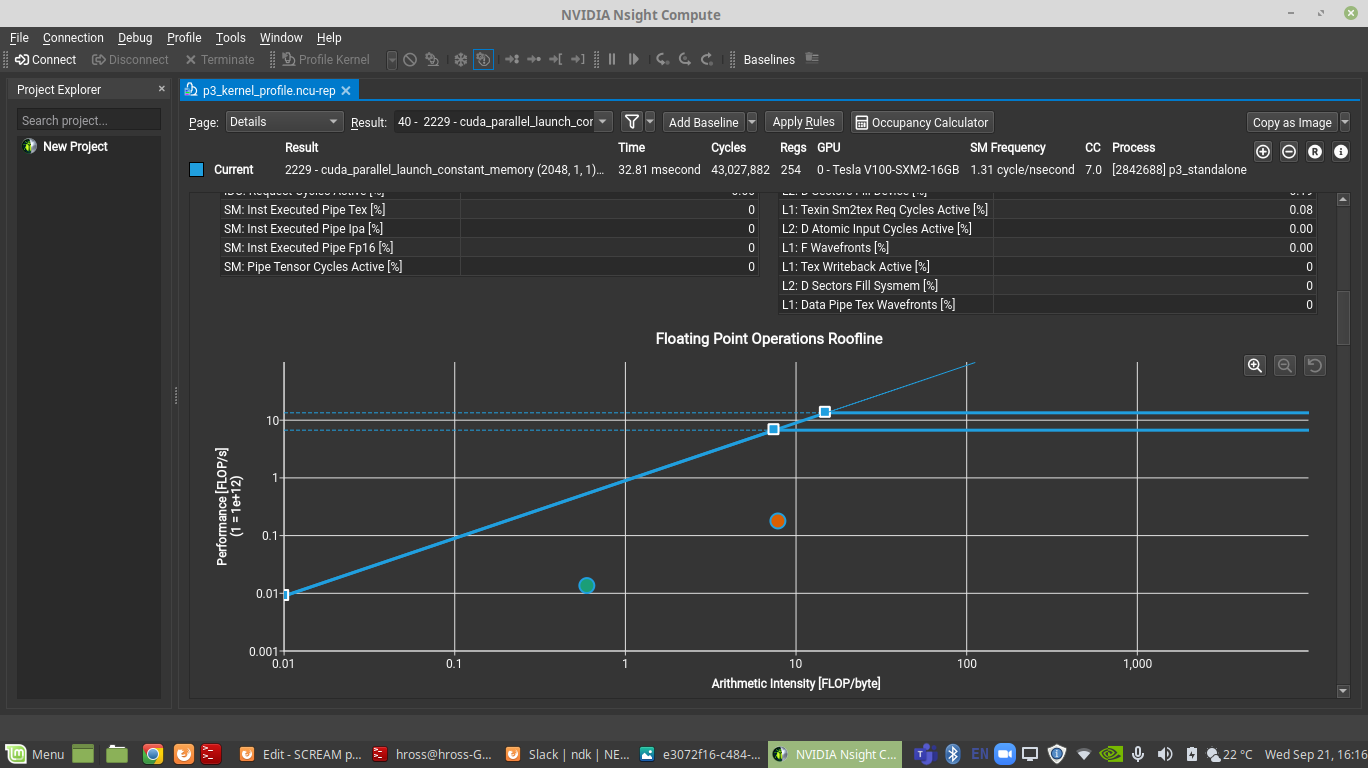
• Arithmetic Intensity: The ratio of floating-point operations to bytes of data moved.
• Memory-Bound: Performance is limited by how fast you can feed the compute units with data from memory. To improve, you need to reduce data movement.
• Compute-Bound: Performance is limited by the raw processing power of the SMs. To improve, you need to use more efficient instructions or increase parallelism.

Case Study: Diagnosing Bottlenecks in FlashAttention

To see ncu in action, we'll follow a real-world investigation from an expert developer who reimplemented FlashAttention and used ncu to systematically find and fix bottlenecks. This is a masterclass in kernel profiling.

This case study perfectly illustrates the iterative process of profiling:

1. Profile with ncu.
2. Identify the primary bottleneck (e.g., HBM bandwidth).
3. Refactor the code to address it.
4. Profile again.
5. Identify the next bottleneck (e.g., shared memory bank conflicts).
6. Repeat.

This process continues until performance is satisfactory or you are verifiably hitting the theoretical limits of the hardware. ncu is the tool that makes this data-driven approach possible.

Another common bottleneck you'll encounter are host-device synchronizations, which can destroy performance by forcing the GPU to wait. The following video explains how to spot and eliminate them.

Conclusion

You have now moved from a high-level understanding of GPU execution to the most granular level of kernel analysis. You're equipped with the same tools and workflow used by performance engineers at NVIDIA and in top AI labs.

Key Takeaways:

• Top-Down Profiling: Use Nsight Systems (nsys) first to get a system-wide view and identify the most time-consuming kernels.
• Deep-Dive Analysis: Use Nsight Compute (ncu) to analyze those top kernels. Start with the roofline model to determine if they are compute- or memory-bound.
• Iterative Optimization: ncu provides specific, actionable metrics (e.g., memory traffic, occupancy, warp stalls, bank conflicts) that guide your code refactoring. The process is a loop: profile, analyze, fix, and repeat.
• Connecting Code to Hardware: The ultimate goal is to understand how your high-level Python/Triton code translates into low-level hardware behavior. Tools like ncu and the ability to inspect PTX assembly make this connection explicit.

Preview of the Next Lesson:

Our deep dive into profiling has repeatedly shown that for LLMs, performance is often dominated by memory access patterns. In the next module, we will focus on the most critical component of a transformer in this regard: the attention mechanism. We will begin by profiling the standard scaled dot-product attention and using ncu to identify its memory-access bottleneck. This will set the stage for understanding FlashAttention, an algorithm specifically designed to be "profiler-friendly" by minimizing costly reads and writes to HBM.