GPU Roofline Model for Performance Analysis

Introduction

Welcome to our next lesson. In the previous session, we did the foundational work of calculating the arithmetic intensity (AI) for the core operations within a transformer. You learned how to derive the FLOPs / Bytes ratio for linear layers and attention mechanisms, establishing that this ratio—the x-axis of a performance plot—is a property of the algorithm itself.

Today, we complete the picture by introducing the Roofline Model. This powerful conceptual tool combines an algorithm's arithmetic intensity with a specific GPU's hardware characteristics—its peak computational performance and memory bandwidth. By the end of this lesson, you will be able to construct and interpret a roofline model to definitively diagnose whether a given operation, running on a specific piece of hardware, is limited by computation speed or memory access speed. This skill is the cornerstone of performance engineering for LLMs.

The Roofline Model: A Framework for Performance

At its core, the Roofline model provides a visual and mathematical answer to the question: "How fast can my code run on this hardware?" It elegantly simplifies a complex system into two primary constraints: compute power and memory bandwidth.

To get a quick but formal introduction to the model, let's watch a brief video.

To summarize the key ideas from the video:

1. The performance of any operation, measured in FLOPs per second (FLOPS), is plotted on the y-axis.
2. The operation's Arithmetic Intensity (AI), measured in FLOPs per Byte, is plotted on the x-axis.
3. The hardware imposes two fundamental limits, or "roofs":
   • A Compute Roof: A horizontal line representing the GPU's theoretical peak performance (P_peak). You can't compute faster than this, no matter how efficient your algorithm is.
   • A Memory Roof: A slanted line with a slope equal to the GPU's memory bandwidth (B_s). For a given AI, your performance is limited by how quickly you can supply the compute units with data. The performance bound is AI * B_s.

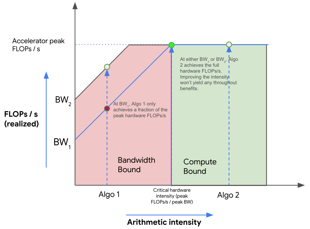
The achievable performance is therefore the minimum of these two constraints. This relationship gives us the iconic roofline plot.

The Ridge Point: A Hardware's Fingerprint

The most important feature of a roofline plot is the "knee" or ridge point where the memory roof meets the compute roof. This point represents the minimum arithmetic intensity an algorithm must have to fully saturate the GPU's compute units.

We can calculate the AI at this ridge point by setting the two performance bounds equal to each other:

This value, AI_critical, is an intrinsic property of the hardware. It's the hardware's own ops:byte ratio. This single number serves as our decision boundary:

• If AI_operation < AI_critical, the operation is memory-bound. Its performance is limited by the slanted memory roof.
• If AI_operation > AI_critical, the operation is compute-bound. Its performance is limited by the horizontal compute roof.

Let's make this concrete by calculating AI_critical for a modern data center GPU, the NVIDIA H100 (SXM variant).

As the resource explains, we find the following from the H100 specifications:

• Peak BF16 Performance (P_peak): 1,979 TFLOPS (with sparsity). Without sparsity, the effective performance is half of this, so 989.5 TFLOPS/s or $9.895\times 10^{14}$ FLOPs/s.
• Memory Bandwidth (B_s): 3.35 TB/s or $3.35\times 10^{12}$ Bytes/s.

Now, we can calculate the H100's critical arithmetic intensity:

This means any operation on an H100 GPU with an arithmetic intensity below ~295 FLOPs/Byte will be bottlenecked by memory bandwidth, leaving the powerful compute cores underutilized.

Case Study: Analyzing Llama-2 on an NVIDIA A6000

Now we can combine the concepts from our last two lessons. We know how to calculate an operation's AI, and we know how to find a hardware's critical AI. Let's analyze a real-world scenario.

The following research paper provides a detailed roofline analysis of Llama-2-7B's layers running on an NVIDIA A6000 GPU.

Table 1 from the paper is a powerful illustration. Let's analyze its findings:

• Prefill Stage (Processing the initial prompt):

  • The linear projections (q_proj, k_proj, v_proj, FFN layers) have an extremely high AI (~1024-1215 FLOPs/Byte). This is far above the GPU's critical AI, making them strongly compute-bound. This aligns with our finding from the last lesson that AI_linear ≈ B, where B is the large prompt length.
  • The matrix multiplications for attention (qk_matmul, sv_matmul) have a lower AI (~114 FLOPs/Byte). On the A6000 (which has a critical AI around 200), this makes them memory-bound, even during prefill.
  • Operations like softmax, norm, and add have very low AI (< 2) and are deeply memory-bound.

• Decode Stage (Generating one token at a time):

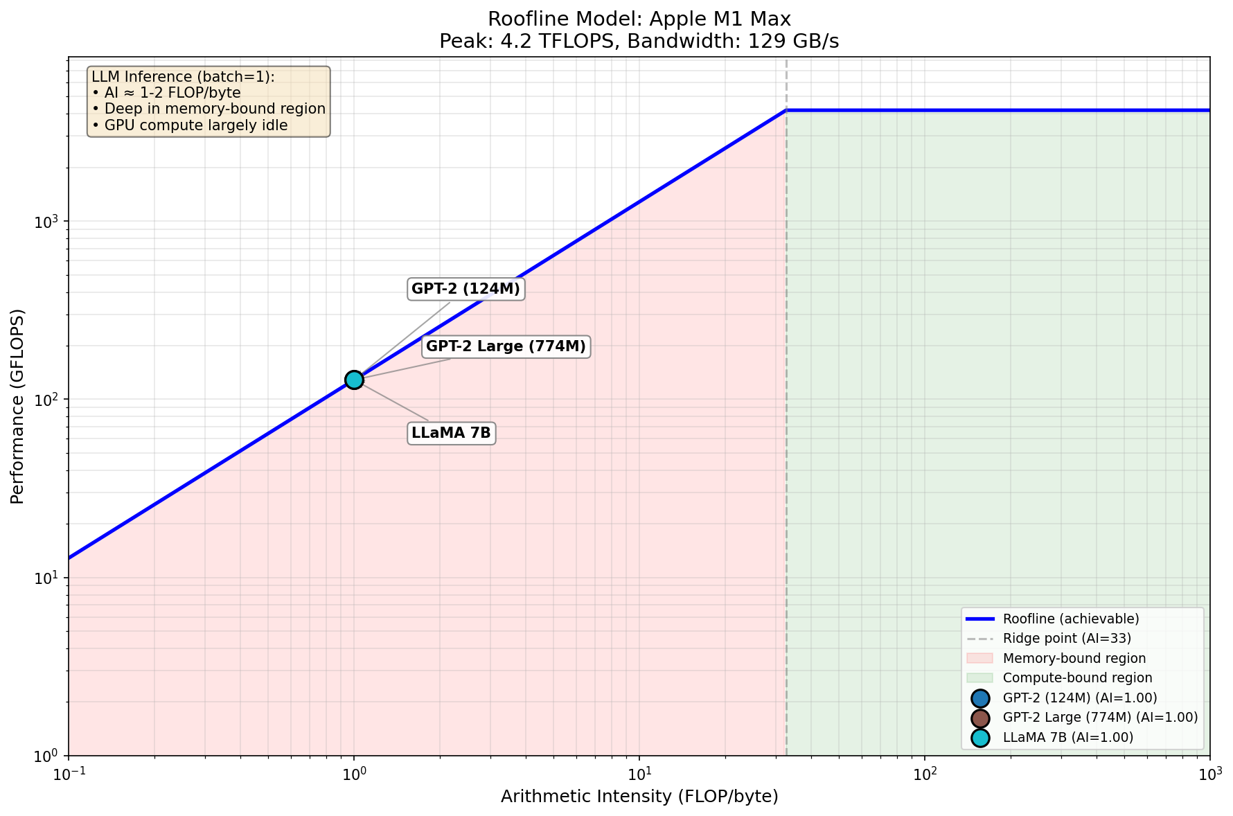
  • Every single operation has an arithmetic intensity of approximately 1-2 FLOPs/Byte.
  • This is far below the hardware's critical AI. Therefore, the entire decode phase is overwhelmingly memory-bound.

This analysis directly answers why LLM inference can be slow despite massive GPU compute power. During the token-by-token generation phase, the GPU isn't waiting on matrix multiplication units; it's waiting for data (weights and the KV cache) to be moved from the main GPU memory (HBM) to the on-chip compute cores (SRAM).

This image provides another visual example, plotting several LLM inference workloads on an Apple M1 Max GPU's roofline.

From Diagnosis to Treatment

Identifying a bottleneck is the first step toward optimization. The roofline model tells us where to focus our efforts.

• If an operation is memory-bound, simply making the compute units faster or using a GPU with a higher P_peak will have little effect. Instead, you need to improve the arithmetic intensity. Techniques like operator fusion do this by combining multiple operations into a single GPU kernel, reducing the total data traffic to and from HBM. We'll explore this in detail in a future lesson.

• If an operation is compute-bound, you can gain performance by using a GPU with higher P_peak or by using lower-precision arithmetic (e.g., INT8 instead of FP16), as this often increases the effective FLOPs rate of the hardware.

Conclusion

In this lesson, you have learned to wield the roofline model as a primary tool for performance analysis. By combining algorithmic properties (arithmetic intensity) with hardware specifications (peak FLOPs and bandwidth), you can now predict and explain the performance of transformer operations.

Key Takeaways:

• The Roofline model visualizes performance as a function of arithmetic intensity, bounded by the hardware's compute and memory roofs.
• A hardware's critical intensity (AI_critical = P_peak / B_s) is the watershed line between being compute-bound and memory-bound.
• You can diagnose a bottleneck by comparing an operation's AI to the hardware's AI_critical.
• In LLM inference, the decode stage is almost always memory-bound due to its low, B=1 arithmetic intensity.
• The prefill stage is a mix, with large linear layers often being compute-bound while attention and element-wise operations can remain memory-bound.

Preview of the Next Lesson:

Now that we can diagnose a memory-bound operation, our next step is to treat it. In the next lesson, we will begin exploring compute optimization by implementing operator fusion. You will see firsthand how combining GPU kernels can reduce memory traffic, increase arithmetic intensity, and improve the performance of memory-bound operations.