Implementing Region-Based CNNs for Object Detection

Hello! Welcome to the first lesson in our module on Advanced Computer Vision Applications.

Introduction

In the previous module, we delved into the powerful building blocks of modern Convolutional Neural Networks, from residual connections to attention mechanisms. Now, we'll see how these components are assembled into sophisticated systems to solve complex, high-level vision tasks.

Our first challenge is object detection, which involves not only classifying what is in an image but also localizing where it is with a bounding box. This lesson focuses on a foundational family of models for this task. Your learning outcome is to implement region-based CNNs (R-CNN, Fast R-CNN, Faster R-CNN) for object detection.

We will trace the evolution of these models, understanding how each iteration solved a critical bottleneck in its predecessor:

R-CNN: The pioneering but slow multi-stage approach.
Fast R-CNN: The first step towards an integrated, faster model.
Faster R-CNN: The breakthrough that introduced a learnable region proposal mechanism, creating a nearly end-to-end system.

This journey highlights a key theme in deep learning engineering: identifying performance bottlenecks and redesigning architectures for more integrated, efficient, and end-to-end solutions.

The Evolution of Region-Based Detectors

The core idea behind Region-based CNNs (R-CNNs) is a two-step process: first, propose a set of candidate regions in the image that might contain an object, and second, classify each of these regions. The evolution of the R-CNN family is a story of optimizing and integrating these two steps.

Comparison of R-CNN, Fast R-CNN, and Faster R-CNN Architectures and Performance — This diagram illustrates the architectural shift and performance gains from R-CNN to Faster R-CNN. Notice how components become more integrated and test time drops dramatically.

1. R-CNN: A Slow Start

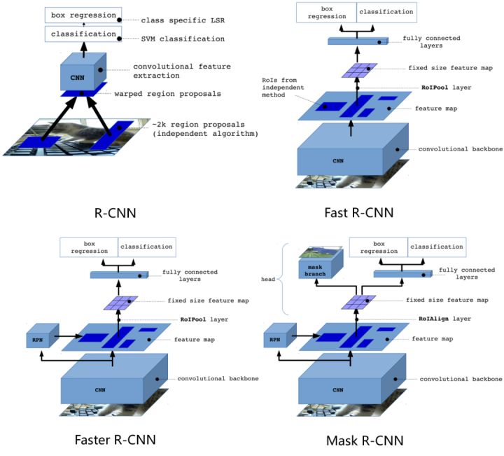
The original R-CNN (Regions with CNN features) laid the groundwork but was notoriously slow and cumbersome. Its process involved several disconnected stages:

Region Proposal: Use an external algorithm, like Selective Search, to generate ~2000 candidate "regions of interest" (RoIs) per image.
Feature Extraction: For each of these ~2000 proposals, independently warp the image patch to a fixed size (e.g., 224x224) and feed it through a CNN (like AlexNet) to extract features.
Classification: Feed the extracted features for each region into a set of linear Support Vector Machines (SVMs), one for each class, to determine if an object is present.
Bounding Box Regression: Train a separate linear regression model to refine the coordinates of the proposed bounding box for a tighter fit.

The primary bottleneck was step 2. Running a powerful CNN on ~2000 overlapping image patches per image was computationally prohibitive, taking nearly a minute per image. The training process was also complex, involving separate training for the CNN, the SVMs, and the regression models.

2. Fast R-CNN: Sharing Computation

Fast R-CNN introduced a crucial optimization that dramatically sped up the process. Instead of running a CNN on every single region proposal, it does the following:

Shared Feature Extraction: Run the entire image through the backbone CNN once to get a single, rich feature map.
Project RoIs: Project the ~2000 region proposals (still generated by Selective Search) onto this feature map.
RoI Pooling: For each projected region, use a special pooling layer called RoI Pooling to extract a fixed-size feature vector (e.g., 7x7) from the corresponding area of the feature map. This solved the problem of handling variable-sized regions.
Unified Head: Feed each fixed-size feature vector into a single network head with two sibling branches: a softmax classifier (replacing the SVMs) and a bounding-box regressor.

This design allowed the model (except for region proposal) to be trained end-to-end with a multi-task loss. By sharing the most expensive part of the computation—the convolutional backbone—Fast R-CNN was orders of magnitude faster than R-CNN. However, the external Selective Search algorithm now became the new bottleneck.

3. Faster R-CNN: Making the Network Propose Regions

The final leap in this family was to eliminate the external region proposal algorithm and have the network learn to propose regions itself. This was the key innovation of Faster R-CNN, achieved by introducing the Region Proposal Network (RPN).

Architectural Comparison of R-CNN, Fast R-CNN, Faster R-CNN, and Mask R-CNN — This diagram shows the architectural progression from R-CNN to Faster R-CNN (and its successor, Mask R-CNN). The key change in Faster R-CNN is the replacement of the "Region proposals" block with the integrated "RPN".

The Region Proposal Network (RPN)

The RPN is a small, fully convolutional network that takes the feature map from the backbone and outputs a set of rectangular object proposals, each with an "objectness" score.

To understand how it works, let's watch a short conceptual overview.

Faster R-CNN: Faster than Fast R-CNN!

The video 'Faster R-CNN: Faster than Fast R-CNN!' by Soroush Mehraban provides an excellent high-level explanation of the motivation for the RPN and how it uses anchor boxes.

Please watch from the beginning to 9:06. Focus on: How the RPN replaces the slow Selective Search algorithm. The concept of anchor boxes: predefined boxes of various scales and aspect ratios that act as references. How the RPN slides over the feature map and, for each location, predicts two things for k anchor boxes: A 2k classification score (object vs. background for each anchor). A 4k regression output (refinements to each anchor's coordinates). The multi-task loss function and the challenge of imbalanced data (many more negative anchors than positive ones).

By integrating the RPN, the entire object detection pipeline becomes almost fully unified within a single network. The RPN and the Fast R-CNN detector share the same convolutional backbone, making the whole system highly efficient and trainable end-to-end.

The complete flow is:

A backbone CNN extracts a feature map from the input image.
The RPN uses this feature map to generate region proposals.
An RoI Pooling layer extracts fixed-size features for each proposal.
A final detector head classifies the proposals and refines their bounding boxes.

Implementation Deep Dive

Given your software engineering background, diving into a from-scratch implementation will solidify your understanding. We will use a detailed PyTorch implementation walkthrough as our main guide. The structure of the code, with its distinct modules for the RPN and RoI Head, is a great example of building a complex deep learning system.

First, let's get an overview of the modules we'll be building.

Faster R-CNN PyTorch Implementation

The video 'Faster R-CNN PyTorch Implementation' by ExplainingAI breaks the model into three clean modules: the Backbone, the Region Proposal Network (RPN), and the RoI Head. Let's start with the high-level architecture.

Watch from 1:45 to 4:29. This segment outlines the overall data flow between the main components, which we will implement step-by-step.

Implementing the Region Proposal Network (RPN)

The RPN is the most novel part of Faster R-CNN. Its implementation involves several key steps: generating anchors, passing features through the RPN's conv layers, creating proposals, and calculating losses for training.

Faster R-CNN PyTorch Implementation

Now, let's dive into the detailed implementation of the RPN. This is the longest and most complex part, so pay close attention to the logic.

Watch from 4:11 to 38:58. This is a dense section, so focus on understanding the purpose of each major block of code: Anchor Generation: How a small set of base anchors (defined by scales and aspect ratios) are tiled across the entire feature map to create thousands of candidate anchors. This is a pure coordinate manipulation task. Applying Predictions: How the 4k regression outputs from the RPN are used to transform the static anchor boxes into proposal boxes. Filtering Proposals: The process of clipping boxes to the image boundary, performing Non-Maximum Suppression (NMS) to remove redundant overlapping proposals, and keeping the top-N scoring ones. Target Assignment (for training): The crucial logic for assigning labels to anchors. An anchor is labeled 'positive' (1) if its IoU with a ground truth box is > 0.7, 'negative' (0) if < 0.3, and ignored otherwise. This step also generates the regression targets. Sampling and Loss Calculation: How a balanced mini-batch of 256 anchors (128 positive, 128 negative) is sampled to compute the classification (binary cross-entropy) and regression (smooth L1) losses.

Test your understanding!

In the RPN training process, why is regression loss (like Smooth L1 loss) only calculated for positive anchors, while classification loss is calculated for both positive and negative anchors?

Show answer

The regression loss's purpose is to train the network to adjust an anchor box to better fit a ground-truth object. This only makes sense if the anchor actually corresponds to an object (i.e., it's a positive anchor). Trying to "regress" a negative anchor (which corresponds to the background) towards a non-existent object is meaningless.

The classification loss, on the other hand, needs both positive and negative examples. The network must learn to distinguish anchors that contain objects from those that are just background.

Implementing the RoI Head (The Detector)

The RoI Head functions as the Fast R-CNN detector, taking the proposals generated by the RPN as input.

Faster R-CNN PyTorch Implementation

With proposals from the RPN, we can now build the final detector, or RoI Head. This part is responsible for the final classification and bounding box refinement.

Watch from 38:41 to 55:37. This segment mirrors the RPN's training logic in many ways, but with a key difference in its goal: Target Assignment: Assigning proposals to ground-truth objects and giving them a specific class label (e.g., 'car', 'person', 'background'), not just 'object' or 'not object'. Sampling: Creating a mini-batch of proposals, again balanced between foreground (positive) and background (negative) examples. RoI Pooling: Using the roi_pool operation to extract a fixed 7x7 feature map for each sampled proposal. Head Layers: Passing the pooled features through fully connected layers to get the final outputs: class scores for C+1 classes (including background) and bounding box regression parameters. Loss Calculation: Computing classification loss (Cross-Entropy) and regression loss (Smooth L1) for the final predictions.

Assembling the Full Model

Finally, a top-level class integrates the backbone, RPN, and RoI Head into a single FasterRCNN model.

Faster R-CNN PyTorch Implementation

Let's see how all the pieces are connected in the main FasterRCNN module.

Watch from 55:21 to 1:03:26. This section covers the end-to-end forward pass, image pre-processing (resizing and normalization), and how the model handles both training and inference modes.

For additional reference, this GitHub repository and Medium article provide excellent supplementary material, including discussions on common implementation pitfalls.

Faster R-CNN in PyTorch and TensorFlow 2 w/ Keras

The README of this GitHub repository, 'Faster R-CNN in PyTorch and TensorFlow 2 w/ Keras', contains valuable insights gained from a from-scratch implementation. The 'Development Learnings' section is particularly insightful for an engineer.

First, briefly scan the 'Background Material' section to see the original research papers that form the basis of these models. Then, carefully read the 'Development Learnings' section. Pay close attention to the two main points, as they address common, non-obvious bugs: Use Object and Background Proposals for Training: Why you must pass the top-N proposals from the RPN to the detector, regardless of their 'objectness' score. Anchor Label Quality: How sensitive the anchor labeling process can be to floating-point precision and implementation details.

Conclusion

In this lesson, we traced the critical evolution of region-based object detectors. We saw how the field moved from a slow, multi-stage pipeline to a fast, elegant, and nearly end-to-end deep learning system.

Key Takeaways:

R-CNN introduced the "propose then classify" paradigm but was slow due to redundant feature computations.
Fast R-CNN optimized this by sharing a single convolutional feature map across all proposals, using RoI Pooling to handle variable-sized regions. Its bottleneck was the external region proposal method.
Faster R-CNN achieved a major breakthrough by replacing the external proposal method with the Region Proposal Network (RPN), a learnable component that generates proposals from the shared feature map using a system of anchor boxes.
The final model is trained with a multi-task loss that combines the losses from both the RPN (objectness classification and box regression) and the final detector (class classification and box regression).

Preview of the next lesson:
While Faster R-CNN is powerful, its two-stage nature (propose, then classify) still has overhead. In the next lesson, we will explore a different family of object detectors: single-shot detectors. We will implement and analyze models like YOLO (You Only Look Once) and SSD (Single Shot MultiBox Detector), which discard the region proposal stage entirely and predict bounding boxes and classes directly in a single pass, enabling real-time performance.