Hello! Welcome back to our course.
Introduction
In our last lesson, we explored the family of two-stage object detectors—R-CNN, Fast R-CNN, and Faster R-CNN. We saw how their "propose-then-classify" strategy, while accurate, involves multiple steps. The final model, Faster R-CNN, integrated the proposal step into the network, but the two-stage nature remains.
Today, we shift our focus to a different paradigm designed for speed and real-time applications: single-shot detectors. Your learning outcome is to implement single-shot detectors (YOLO, SSD) for real-time object detection. These models discard the separate region proposal stage and instead perform localization and classification in a single forward pass of the network.
We will cover two seminal single-shot architectures:
- YOLO (You Only Look Once): Which introduced the clever idea of framing object detection as a regression problem on a grid.
- SSD (Single Shot MultiBox Detector): Which combined the single-shot approach with ideas from Faster R-CNN, like anchor boxes, and introduced predictions over multi-scale feature maps to improve performance on objects of various sizes.
This lesson will focus on the core architectural ideas and the implementation of their key components, particularly their unique network outputs and loss functions.
1. YOLO: You Only Look Once
The first version of YOLO proposed a radically different and simpler approach. Instead of a complex pipeline, it treats object detection as a single regression problem, straight from image pixels to bounding box coordinates and class probabilities.
The Core Idea: A Grid-based Approach
YOLO divides the input image into an S x S grid. If the center of an object falls into a grid cell, that grid cell is "responsible" for detecting that object. For each grid cell, the model predicts:
Bbounding boxes and a confidence score for each box. The confidence score reflects how confident the model is that the box contains an object and how accurate it thinks the box is.Cclass probabilities, conditional on an object being present.
Let's watch a short video that visualizes this core concept.
The video 'YOLOv1 from Scratch' by Aladdin Persson provides an excellent explanation of the fundamental idea behind YOLOv1. Pay close attention to how the image is divided into a grid and what each grid cell is responsible for predicting.
Watch from 01:15 to 07:49. Focus on: How the image is divided into an S x S grid (e.g., 7x7 in the paper). The concept of the 'responsible' grid cell, determined by the object's midpoint. The structure of the output tensor for each cell: (x, y, w, h, confidence) for each bounding box, plus class probabilities. A key limitation: each grid cell can only predict one class, making it difficult to detect multiple small objects in the same cell.
This leads to a final output tensor of shape S x S x (B * 5 + C). For the original YOLO paper, this was 7 x 7 x (2 * 5 + 20) = 7 x 7 x 30.
YOLOv1 Architecture and Implementation
The YOLOv1 network, nicknamed "Darknet," is a straightforward convolutional neural network inspired by GoogLeNet. It consists of convolutional layers followed by fully connected layers.
A clever way to implement such an architecture, especially when translating from a research paper, is to define the layers in a configuration list. This makes the code clean and easy to modify.
Let's continue with the same video to see how the architecture from the YOLO paper is translated into a Python configuration that can be used to build the model in PyTorch.
Watch from 07:49 to 14:00. You don't need to follow every line of the live coding, but focus on how the author: Walks through the architecture diagram from the paper. Creates a Python list of tuples (architecture_config) to represent the sequence of convolutional and max-pooling layers. Plans to write a helper function (_create_conv_layers) to parse this configuration and build the nn.Sequential model. This is a common and effective pattern in software engineering for deep learning.
As you saw, the core of the implementation involves parsing that configuration list. The video goes on to implement this in detail. The main logic resides in a loop that iterates through the architecture_config. Based on the type of element (tuple for a conv layer, string for a max-pool, list for a repeated block), it appends the corresponding PyTorch module to a layers list, which is finally passed to nn.Sequential. This is a powerful technique for building complex, bespoke architectures from a declarative format.
The YOLOv1 Loss Function
The loss function is the most complex part of YOLOv1. It's a multi-part, sum-squared error loss that combines several objectives.
- Localization Loss (Coordinate Loss): Penalizes errors in the predicted bounding box coordinates (
x, y, w, h). It only applies if an object is present in a grid cell. - Confidence Loss (Objectness Loss): This has two parts:
- If an object is present, it pushes the confidence score of the "responsible" box towards 1.
- If an object is not present, it pushes the confidence scores of all boxes in that cell towards 0.
- Classification Loss: If an object is present, it penalizes errors in the class probabilities.
The total loss is a weighted sum of these components. The weights, λ_coord and λ_noobj, are crucial. λ_coord is set high (e.g., 5) to emphasize correct localization, while λ_noobj is set low (e.g., 0.5) to down-weight the loss from the vast majority of grid cells that contain no objects.
Now, let's understand this complex loss function. The video provides a clear breakdown of each component directly from the paper's equation.
Watch from 31:53 to 38:30. Focus on understanding the purpose of each of the five terms in the loss function equation: XY Loss: For the center coordinates of the responsible box. WH Loss: For the width and height. Note the use of the square root to handle large vs. small boxes more equally. Object Confidence Loss: For positive predictions. No-Object Confidence Loss: For negative predictions (penalizes both box predictors). Class Loss: For class probabilities.
Implementing this in PyTorch involves careful tensor manipulation to isolate the positive ("object-present") and negative ("no-object") predictions and apply the correct loss to each part. The concept of the "responsible" bounding box predictor (the one with the highest IoU with the ground truth) is key to only penalizing one box for localization and objectness per object.
2. SSD: Single Shot MultiBox Detector
While YOLO was groundbreaking, it had notable weaknesses, particularly in detecting small objects and objects that were close together. The Single Shot MultiBox Detector (SSD) was proposed shortly after and offered a more robust single-shot solution by incorporating ideas from two-stage detectors like Faster R-CNN.
Core Concepts of SSD
Let's begin with a short reading to define the key concepts behind SSD.
The GitHub repository 'a-PyTorch-Tutorial-to-Object-Detection' provides a fantastic written tutorial on SSD. We'll start with the 'Concepts' section to get a solid grasp of the terminology.
Read the section titled 'Concepts'. Focus on the definitions of: Single-Shot Detection: Encapsulating localization and detection in a single forward sweep. Multiscale Feature Maps: Using feature maps from different layers to detect objects of various sizes. Priors: Pre-computed boxes that serve as anchors or reference points for predictions (very similar to the anchor boxes in Faster R-CNN's RPN). Multibox: Formulating box prediction as a regression problem relative to these priors. Hard Negative Mining: A strategy to deal with the extreme imbalance between negative (background) and positive (object) examples.
SSD's two main innovations are:
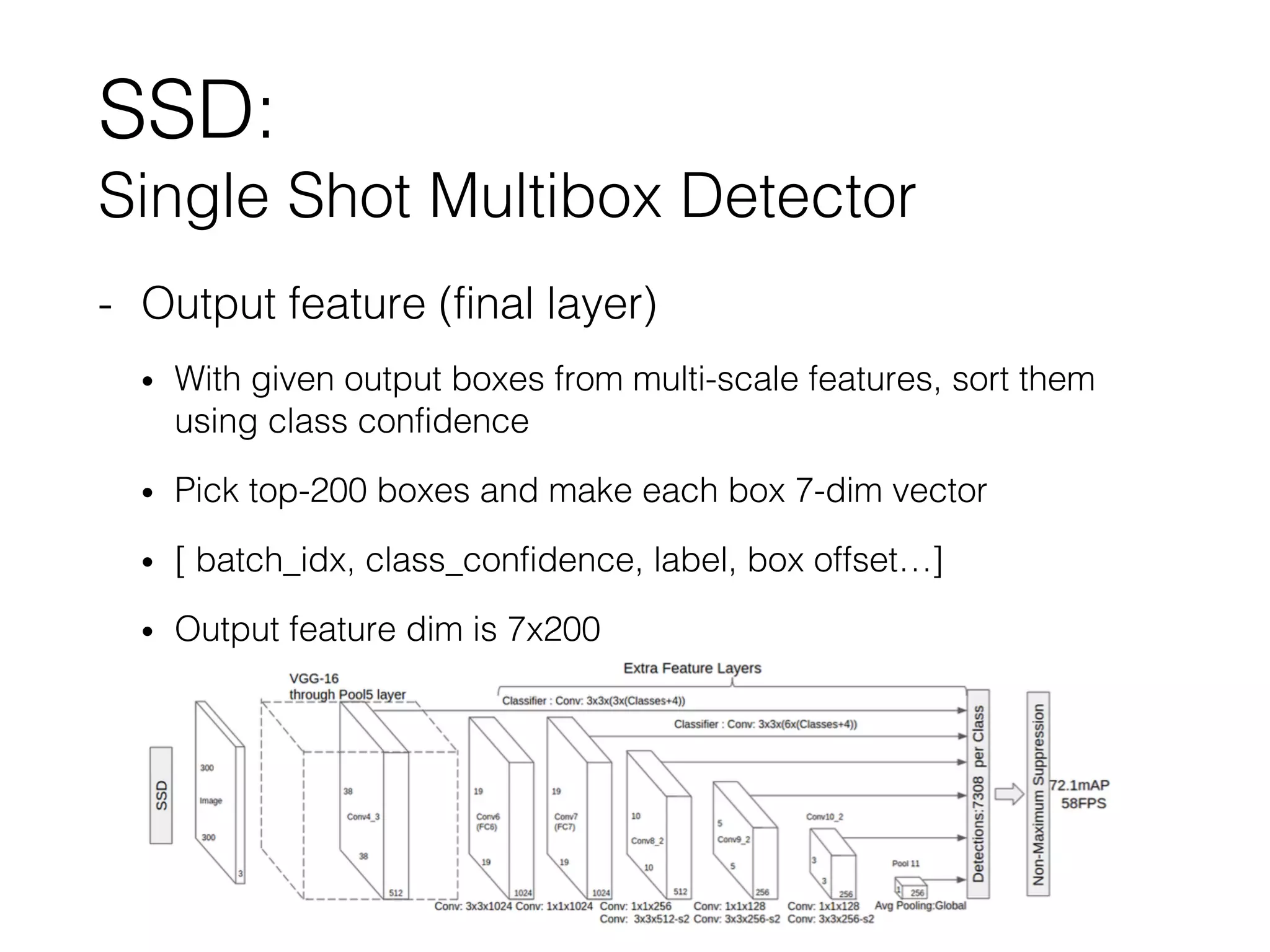
- Multi-scale Feature Maps: Unlike YOLOv1, which makes all predictions from its final feature map, SSD makes predictions from feature maps at several different stages of the network. Earlier, higher-resolution maps are used to detect small objects, while later, lower-resolution maps are used to detect large objects.
- Default Boxes (Priors): Instead of predicting box coordinates from scratch, SSD uses a set of default boxes with pre-defined aspect ratios and scales at each location on these feature maps. The network then predicts offsets relative to these default boxes, along with class scores. This makes the regression task much easier for the network to learn.
This video provides an excellent walkthrough of these core SSD concepts.
Single Shot Multibox Detector | SSD Object Detection Explained and Implemented
The video 'Single Shot Multibox Detector | SSD Object Detection Explained and Implemented' by ExplainingAI offers a clear, conceptual walkthrough of SSD's architecture and mechanics.
Please watch from the beginning to 17:17. This covers three key parts: (0:00 - 2:37) Introduction to SSD and the parallel between its 'default boxes' and Faster R-CNN's 'anchor boxes'. (2:37 - 12:18) The crucial idea of using multiple feature maps and the formulation for calculating the scales and aspect ratios of the default boxes. (12:18 - 17:17) The matching strategy (how default boxes are matched to ground truths) and the loss function, including the use of Hard Negative Mining to address class imbalance.
Test your understanding!
What problem does "Hard Negative Mining" solve in the context of SSD? Why is it necessary?
Show answer
In SSD, thousands of default boxes are generated across the image. The vast majority of these will not overlap with any ground-truth object, making them "negative" examples (background). If all these negatives were used for training, they would overwhelm the handful of "positive" examples (the boxes that do contain objects). This imbalance would cause the model to become very good at predicting "background" and terrible at predicting actual objects.
Hard Negative Mining addresses this by selecting only the "hardest" negative examples for training—specifically, the negative boxes that the model was most confident were objects (i.e., those with the highest confidence loss). By focusing on these mistakes, the model learns to be a better classifier without being overwhelmed by easy negative examples.
SSD Architecture and Loss Function in Detail
To solidify your understanding of the architecture and the loss function, let's turn back to our written resource. It provides a detailed, step-by-step breakdown that complements the video.
SSD - Overview, Priors, and Loss
This reading from 'a-PyTorch-Tutorial-to-Object-Detection' provides a more in-depth look at the SSD architecture, the priors, and the loss function. It's a great way to consolidate what you've learned from the video.
Read through the following three sections: Overview: This breaks the SSD300 model into its three main parts: Base Convolutions, Auxiliary Convolutions, and Prediction Convolutions. It also explains the clever technique of converting fully connected layers (like in VGG) into convolutional layers. A detour (Priors): This section gives a fantastic explanation of what priors are, how they are calculated for different feature maps, and how the model's predictions are just offsets from these priors. Multibox loss: This details the matching process and the two components of the loss: Localization loss (Smooth L1) for positive matches and Confidence loss (Cross-Entropy) for positive and hard-negative matches.
YOLO vs. SSD: The Evolution of Single-Shot Detectors
YOLOv1 and SSD represent two early, foundational approaches to single-shot detection.
- YOLOv1 used a coarse grid and predicted "from scratch," making it very fast but less accurate, especially for small or oddly-shaped objects.
- SSD introduced multi-scale predictions and anchor-like default boxes, making it significantly more accurate and robust across different object scales, while still maintaining high speed.
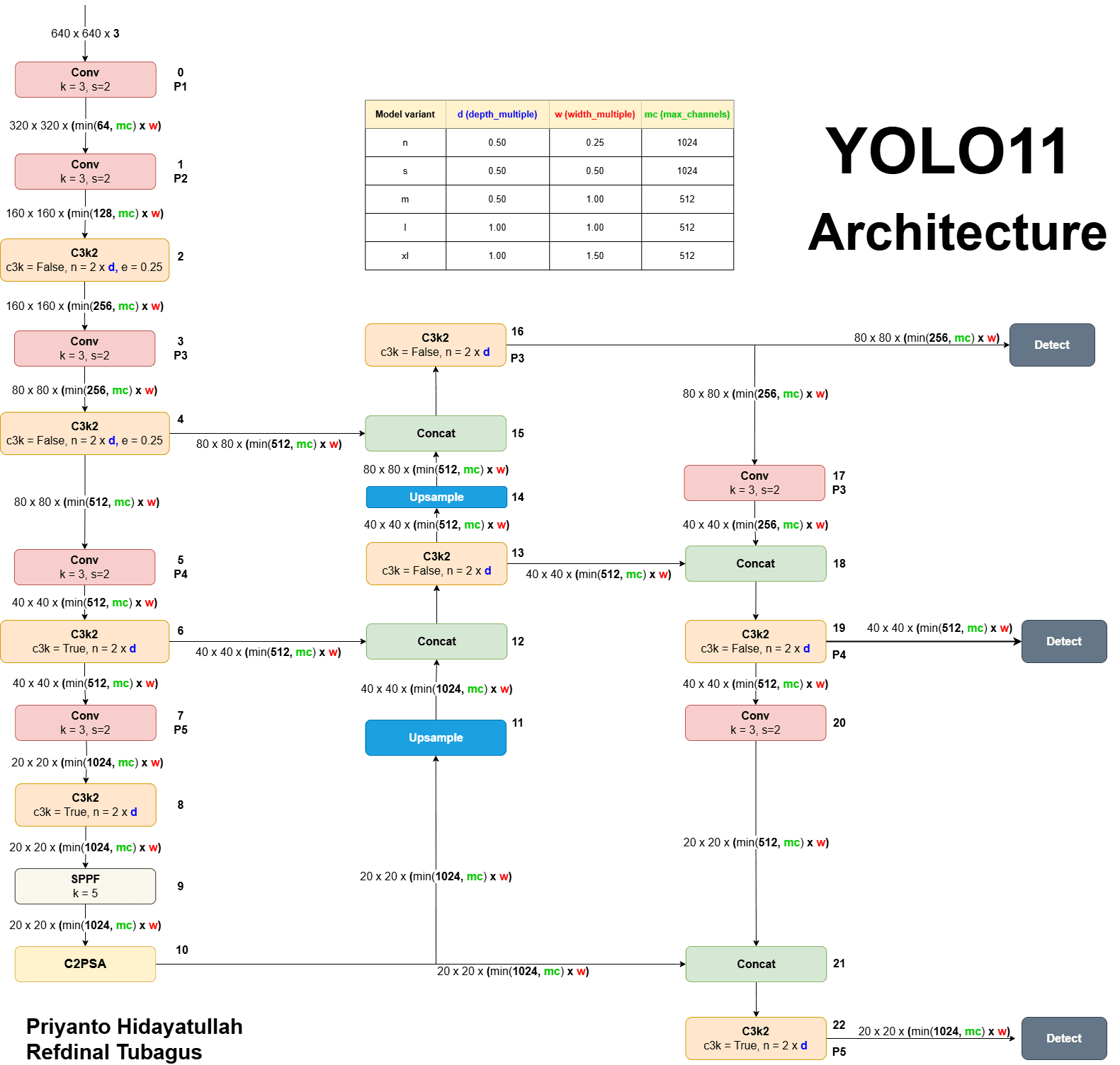
The ideas from SSD proved to be extremely influential. Subsequent versions of YOLO (from YOLOv2 onwards) adopted and refined these concepts, particularly the use of anchor boxes and predictions at multiple scales. Modern YOLO architectures look very different from YOLOv1 and have become a hybrid of the original grid-based idea and the anchor-based, multi-scale approach pioneered by SSD and Faster R-CNN.
Conclusion
In this lesson, we explored the world of single-shot object detectors, which revolutionized the field by enabling real-time performance.
Key Takeaways:
- Single-Shot Paradigm: These detectors combine object localization and classification into a single network pass, eliminating the separate region proposal stage of two-stage models like Faster R-CNN.
- YOLOv1: Introduced the idea of dividing an image into a grid and having each cell regress bounding boxes and class probabilities. It is extremely fast but has limitations with small or overlapping objects.
- SSD: Improved upon YOLO by making predictions from multi-scale feature maps and using default boxes (priors) of different scales and aspect ratios. This significantly improved accuracy, especially for objects of varying sizes.
- Key Techniques: We learned about crucial implementation details like the multi-part loss function in YOLO and the concepts of matching strategies and hard negative mining in SSD.
Preview of the next lesson:
Both YOLO and SSD produce a dense set of thousands of potential bounding boxes. To get to the final, clean detections, a crucial post-processing step is required. In our next lesson, we will dive deep into this step and apply non-maximum suppression (NMS) to refine detection bounding boxes.