Semantic Segmentation with FCNs and U-Net

Hello! Let's dive into our next topic in advanced computer vision.

Introduction

In our recent lessons, we explored object detection, focusing on models like YOLO and SSD that identify objects and draw bounding boxes around them. We concluded by learning how to refine those boxes using Non-Maximum Suppression. Now, we're going to take a step further in understanding image content. Instead of asking "Where is the object?", we'll ask, "To which category does every single pixel in this image belong?"

This task is known as semantic segmentation. Today's learning outcome is to implement fully convolutional networks (FCNs) and U-Net for semantic segmentation. These are two foundational architectures that revolutionized how machines perform this pixel-level classification.

We will cover:

1. The core concept of semantic segmentation.
2. Fully Convolutional Networks (FCNs): The breakthrough that enabled end-to-end pixel-wise prediction.
3. U-Net: A highly influential FCN variant that excels at precise localization by using "skip connections."
4. A from-scratch implementation of U-Net in PyTorch, covering its key building blocks.

By the end of this lesson, you will understand the architectural principles behind modern segmentation models and be able to build one yourself.

1. What is Semantic Segmentation?

Semantic segmentation is the task of classifying each pixel in an image into a specific class. Unlike object detection, which produces bounding boxes, semantic segmentation outputs a dense prediction map, often called a segmentation mask, which has the same dimensions as the input image. In this mask, the value of each pixel corresponds to a class label (e.g., 0 for background, 1 for car, 2 for person).

Let's watch a short video that introduces the concept and its applications.

This pixel-level understanding is crucial for applications requiring precise spatial awareness, such as autonomous driving (identifying road, pedestrians, other vehicles), medical image analysis (delineating tumors or organs), and photo editing (separating a person from the background).

2. Fully Convolutional Networks (FCN)

The pioneering work that enabled modern deep learning-based segmentation was the Fully Convolutional Network (FCN). Before FCNs, classification networks (like VGG or AlexNet) ended with fully connected (dense) layers, which discarded all spatial information and produced a single vector of class probabilities. This was great for classifying an entire image, but useless for pixel-wise tasks.

The key insight of FCNs was to replace the fully connected layers with convolutional layers (specifically, 1x1 convolutions).

This simple change had two profound consequences:

1. The network could now accept inputs of arbitrary size.
2. The output was a spatial feature map (a heatmap), not a 1D vector, preserving spatial dimensions and allowing for pixel-wise predictions.

To learn more about this core idea, please read the following article.

FCNs typically adopt an encoder-decoder structure:

• Encoder (Contracting Path): A standard classification network (e.g., VGG, ResNet) is used to downsample the image and extract hierarchical features. The deeper the layer, the more semantic the information, but the lower the spatial resolution.
• Decoder (Expanding Path): The decoder's job is to upsample the coarse, low-resolution feature maps from the encoder back to the original image resolution to make a pixel-wise prediction. This is often done using transposed convolutions, a type of learnable upsampling layer.

However, a lot of fine-grained spatial information is lost during the encoder's downsampling. This makes it difficult for a simple FCN decoder to produce crisp, precise boundaries. This limitation led to the development of our next architecture.

3. U-Net: Precise Segmentation with Skip Connections

The U-Net architecture, introduced in 2015 for biomedical image segmentation, elegantly solved the problem of lost spatial information. Its main innovation is the use of skip connections.

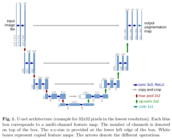
Here's how it works:

1. Encoder (Contracting Path): Similar to an FCN, the encoder consists of repeated blocks of convolutions and max pooling to downsample the input and capture context.
2. Decoder (Expansive Path): The decoder systematically upsamples the feature maps using transposed convolutions.
3. Skip Connections: This is the key. After each upsampling step in the decoder, the resulting feature map is concatenated with the corresponding feature map from the encoder path. These connections bridge the high-resolution, low-level feature maps from the encoder directly to the decoder.

This allows the decoder to use both the deep, semantic information passed up from the bottleneck and the fine-grained, high-resolution information from the skip connections to reconstruct a highly precise segmentation map.

To see this process explained conceptually, let's return to the TileStats video.

Test your understanding!

Why are skip connections so critical for the performance of U-Net, especially for tasks requiring precise boundaries like medical image segmentation?

Show answer

The downsampling operations (max pooling) in the encoder path, while great for capturing semantic context and creating a large receptive field, progressively reduce spatial resolution. This means fine-grained details about object boundaries and textures are lost in the deeper layers. The decoder, working only with the coarse feature maps from the bottleneck, would struggle to reconstruct these details accurately.

Skip connections provide a "shortcut" for the high-resolution feature maps from the encoder to be directly accessed by the decoder. This allows the decoder to combine the "what" information (semantic context from deep layers) with the "where" information (precise localization from shallow layers), enabling it to reconstruct segmentation masks with much sharper and more accurate boundaries.

4. Implementing U-Net from Scratch in PyTorch

Now, let's translate this architecture into code. Given your background, building the model from scratch in PyTorch is the best way to solidify your understanding. We will follow a very clean, modular implementation approach.

The following video provides a complete, line-by-line guide to building, training, and testing a U-Net. We'll focus on the model implementation part.

Code Breakdown and Reinforcement

Let's summarize the key components of the PyTorch implementation you just watched. You can also refer to the code in the article Implementing U-Net from Scratch in PyTorch for Medical Segmentation (resource ID LINK, section Implementing the U-Net Model) for a static view of a similar, slightly more explicit implementation.

1. The DoubleConv Module:
This is a simple nn.Sequential module containing two Conv2d layers, each typically followed by a BatchNorm2d (as in the video) or just a ReLU (as in the original paper). Modularizing this cleans up the main UNet class significantly.

# A simplified version of the DoubleConv block
class DoubleConv(nn.Module):
    def __init__(self, in_channels, out_channels):
        super(DoubleConv, self).__init__()
        self.conv = nn.Sequential(
            nn.Conv2d(in_channels, out_channels, 3, 1, 1, bias=False), # padding=1 for same convolution
            nn.BatchNorm2d(out_channels),
            nn.ReLU(inplace=True),
            nn.Conv2d(out_channels, out_channels, 3, 1, 1, bias=False),
            nn.BatchNorm2d(out_channels),
            nn.ReLU(inplace=True),
        )

    def forward(self, x):
        return self.conv(x)

2. The UNet Forward Pass:
The logic within the forward method is the essence of the architecture.

# Conceptual forward pass
def forward(self, x):
    skip_connections = []

    # --- Encoder Path ---
    # For each downsampling step:
    # 1. Pass input through a DoubleConv block
    # 2. Store the output for the skip connection
    # 3. Apply max pooling to the output
    
    # --- Bottleneck ---
    # Pass through the final DoubleConv at the bottom of the 'U'

    # --- Decoder Path ---
    # For each upsampling step:
    # 1. Apply a transposed convolution to the feature map
    # 2. Get the corresponding skip connection feature map
    # 3. Concatenate them along the channel dimension: 
    #    torch.cat((skip_feature, upsampled_feature), dim=1)
    # 4. Pass the concatenated map through a DoubleConv block
    
    # --- Final Output ---
    # Apply a final 1x1 convolution to map to the number of classes

    return final_output

The concatenation step is where the channel dimensions add up. For example, if an upsampled feature map has 512 channels and the corresponding skip connection from the encoder also has 512 channels, the concatenated tensor will have 1024 channels. This is why the subsequent DoubleConv block in the decoder must have an in_channels of 1024.

The video you watched provides the full, working code for this entire process, including the dataset and training loop, which serves as an excellent practical reference.

Conclusion

Today we made the leap from localizing objects with boxes to understanding images at the pixel level. We dissected two of the most important architectures in semantic segmentation.

Key Takeaways:

• Semantic Segmentation: The task of assigning a class label to every pixel in an image, producing a segmentation mask.
• Fully Convolutional Networks (FCNs): Pioneered end-to-end segmentation by replacing fully connected layers with convolutions, enabling spatial outputs from a deep network.
• U-Net Architecture: Refined the FCN's encoder-decoder design with skip connections, which feed high-resolution feature maps from the encoder to the decoder.
• Skip Connections: This key innovation allows the model to combine high-level semantic information ("what") with low-level spatial detail ("where"), leading to highly precise segmentation boundaries.
• Implementation: U-Net's symmetric and modular structure is well-suited for implementation in frameworks like PyTorch, using Conv2d, MaxPool2d, ConvTranspose2d, and torch.cat.

Preview of the next lesson:
We have now covered object detection (where are the individual objects?) and semantic segmentation (what is each pixel's class?). The next logical step is to combine them. In our next lesson, we will implement Mask R-CNN for instance segmentation. This powerful model performs both tasks simultaneously: it detects each instance of an object and generates a separate segmentation mask for each one. You'll see how it builds directly on the concepts of region-based detectors like Faster R-CNN, which we've discussed previously.