Object Detection & Segmentation Metrics: mAP & IoU

Hello! Let's dive into our next lesson on evaluating computer vision models.

Introduction

In our last lesson, we built a Mask R-CNN model to perform instance segmentation, generating both bounding boxes and pixel-perfect masks for objects in an image. Building the model is only half the battle. How do we objectively measure its performance? How can we tell if one model is better than another, or if our fine-tuning has actually improved anything?

This lesson addresses exactly that. Your learning outcome is to evaluate object detection and segmentation models using appropriate metrics (mAP, IoU). We will deconstruct the industry-standard metric, mean Average Precision (mAP), from the ground up. This metric is the primary benchmark used in academic papers and competitions like COCO.

We will cover the following concepts in order:

1. Intersection over Union (IoU): The fundamental measure of overlap that determines if a single prediction is "correct."
2. Precision and Recall: How these classic classification metrics are adapted for object detection.
3. Average Precision (AP): A single-number score that summarizes a model's performance for a single class.
4. Mean Average Precision (mAP): The final metric, which averages AP across all classes and multiple IoU thresholds to give a comprehensive evaluation of the model.

1. Intersection over Union (IoU): The Atomic Unit of Evaluation

Everything starts with a simple question: for a given object, how well does our model's predicted bounding box (or mask) line up with the ground truth? This is measured by Intersection over Union (IoU).

As the name suggests, IoU is calculated as the ratio of the area of overlap between the predicted and ground truth boxes to the area of their combined union.

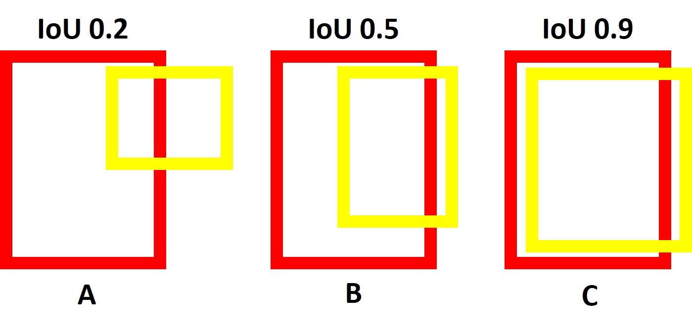
IoU is the foundational metric that allows us to classify a detection as correct or incorrect. We do this by setting an IoU threshold. For example, a common threshold is 0.5. If a predicted box has an IoU with a ground truth box that is greater than or equal to 0.5, we consider it a True Positive (TP). If the IoU is less than 0.5, it's a False Positive (FP).

The same logic applies to segmentation masks. Instead of the area of bounding boxes, we calculate the overlap in terms of pixels.

2. Precision and Recall in Object Detection

With IoU allowing us to count True Positives and False Positives, we can now define Precision and Recall for object detection.

• Precision: Of all the detections our model made, what fraction was actually correct? $$\text{Precision}=\frac{\text{TP}}{\text{TP}+\text{FP}}=\frac{\text{Number of correct detections}}{\text{Total number of detections}}$$
• Recall: Of all the actual objects present in the image, what fraction did our model successfully detect? $$\text{Recall}=\frac{\text{TP}}{\text{TP}+\text{FN}}=\frac{\text{Number of correct detections}}{\text{Total number of ground truth objects}}$$ Here, a False Negative (FN) is a ground truth object that the model failed to detect.

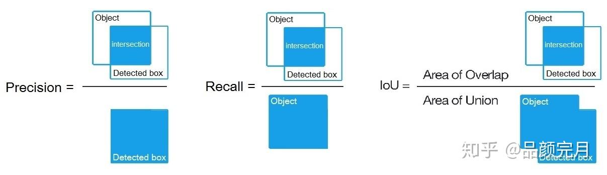
There is a natural trade-off. If we lower our model's confidence threshold, it will produce many more bounding boxes. This will likely increase Recall (we'll miss fewer objects) but decrease Precision (many of the new boxes will be incorrect). The mAP metric is designed to evaluate a model's performance across this entire trade-off.

3. The Path to mAP: Precision-Recall Curve and Average Precision (AP)

To get a single, robust metric, we need to evaluate the model not at a single confidence threshold, but across all possible thresholds. This is done by calculating the Average Precision (AP) for each class.

The calculation of AP is an algorithmic process. For a single class (e.g., "person"):

1. Gather all predicted bounding boxes for that class from every image in your test set. Each prediction has a confidence score.
2. Sort these predictions in descending order of their confidence scores.
3. Iterate down this sorted list. At each prediction, calculate the cumulative Precision and Recall.
4. Plot these Precision vs. Recall values. This creates the Precision-Recall Curve.
5. Average Precision (AP) is the area under this Precision-Recall curve.

A higher AP means the model can maintain high precision even as it achieves high recall, which indicates a high-quality model.

Test your understanding!

In the AP calculation process, why is it necessary to sort the detections by their confidence score before computing the precision-recall curve?

Show answer

Sorting by confidence score simulates moving a decision threshold from high to low. High-confidence predictions are considered first. This allows the precision-recall curve to show how the model's performance changes as we become more lenient and start including lower-confidence detections. A good model will have its true positives ranked with high confidence, leading to high precision at the beginning (low recall) of the curve. Without sorting, the curve would be erratic and wouldn't represent the model's precision/recall trade-off in a meaningful way.

There are different ways to calculate the area under the P-R curve. Older methods used an 11-point interpolation, while modern methods (like the one used in the COCO challenge) compute the exact area using numerical integration.

4. Mean Average Precision (mAP): The Final Score

We now have the Average Precision (AP) for a single class. Mean Average Precision (mAP) is simply the mean of the APs calculated for all classes.

$$\text{mAP}=\frac{1}{N}\sum _{i=1}^N{\text{AP}}_i$$

where $N$ is the number of classes.

But modern evaluation takes it one step further. Remember that our initial TP/FP classification depended on an IoU threshold (e.g., 0.5). A model that is "correct" at IoU=0.5 might be very imprecise at IoU=0.9. To reward models that are accurate at multiple levels of localization, the standard COCO metric calculates mAP over a range of IoU thresholds.

You will often see this written as mAP@[.5:.05:.95]. This means:

1. Calculate the mAP with an IoU threshold of 0.5.
2. Calculate the mAP with an IoU threshold of 0.55.
3. ...and so on, up to an IoU threshold of 0.95.
4. Finally, average all of these mAP scores.

This single number provides a very robust assessment of a model's overall performance.

5. Implementation Deep Dive

Given your background, understanding how this is implemented in code will solidify the concepts. The algorithmic nature of mAP calculation—sorting, iterating, and tracking state—should feel familiar. The Aladdin Persson video continues with a full PyTorch implementation from scratch.

This is the most practical part of the lesson. We will focus on the key logic that translates the theory into code.

Conclusion

You've now covered the entire pipeline for evaluating object detection and instance segmentation models, from the basic concept of IoU to the comprehensive mAP metric.

Key Takeaways:

• IoU is the foundation, measuring the overlap between a single prediction and a ground truth box/mask.
• An IoU threshold is used to classify detections as True Positives or False Positives.
• Precision and Recall capture the trade-off between the quality and quantity of detections.
• The Precision-Recall Curve visualizes this trade-off across all confidence scores.
• Average Precision (AP) is the area under the P-R curve, providing a single-number summary for one class.
• Mean Average Precision (mAP) is the final, robust metric, averaging AP across all classes and typically across a range of IoU thresholds (e.g., mAP@[.5:.05:.95]).

Preview of the next lesson:
We have now completed our deep dive into discriminative models for computer vision, which are trained to recognize patterns and make predictions. We are about to pivot to a completely different and exciting area of AI: generative models. Instead of just analyzing existing data, these models learn to create entirely new data. In our next lesson, we will begin this journey by implementing a Variational Autoencoder (VAE), one of the foundational generative architectures.