Optimizing API Request Latency

Introduction

In our last lesson, you implemented a bounded request queue and a load-shedding mechanism. This was a crucial step in ensuring your service remains stable under high load by gracefully rejecting requests it cannot handle. However, this queue, along with other components like the API server and data processing steps, introduces latency outside of the core model execution on the GPU.

Today, we'll learn how to see the complete picture. Your learning outcome is to profile the full end-to-end API request path to identify and optimize non-inference latency bottlenecks. As GPUs become more powerful, the time spent on the CPU—handling requests, scheduling, and moving data—often becomes the limiting factor for performance. This lesson will equip you with the mental model and practical tools to find and fix these hidden costs.

The Anatomy of End-to-End Latency

When a user interacts with your service, their perceived latency is a sum of many parts. It's not just the time the GPU spends crunching numbers. Let's break it down.

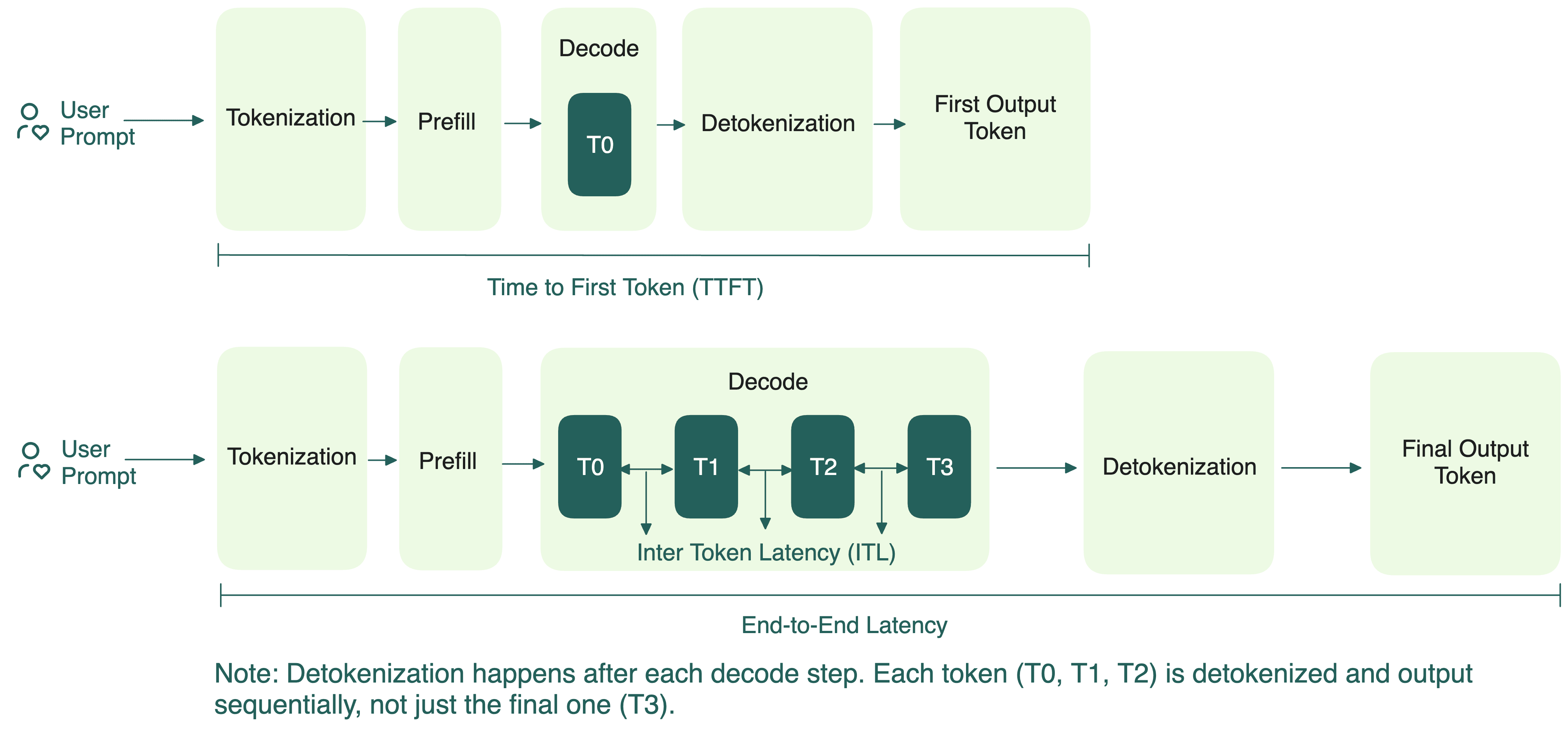
To effectively optimize, we need to dissect these high-level metrics into the constituent stages of our system:

1. Network and API Overhead: Time for the request to travel from the client to your server and for your FastAPI application to receive it, validate it, and parse the JSON payload.
2. Queuing: The time a request spends in the bounded queue you implemented, waiting for the inference engine to become available.
3. Scheduling and Batching: The time your engine's scheduler takes to decide which requests from the queue to group into the next batch.
4. Data Pre-processing: Primarily, tokenizing the input text.
5. GPU Execution (Prefill): The first, compute-intensive forward pass on the user's prompt to generate the KV cache and the first token. This is a major part of TTFT.
6. Data Post-processing and Streaming: Detokenizing the first output token and sending it back to the client.
7. Autoregressive Decode Loop (for subsequent tokens): This loop dominates ITL and consists of smaller, faster steps:
   • Scheduling for the next step.
   • GPU Execution (Decode): A single, faster forward pass to generate one token.
   • Post-processing: Detokenizing, checking stopping conditions, and streaming the token.

To reinforce these concepts, let's watch a short segment that introduces the key performance metrics from a systems perspective.

Understanding this full breakdown is the first step. If TTFT is high, the bottleneck could be a long prompt (heavy prefill), a long queue, or slow API server logic. You can't know which without measuring.

Case Study: Identifying Real-World Bottlenecks

This is not just a theoretical problem. As inference engines have become highly optimized, CPU overhead has emerged as a major performance limiter in real-world systems. The vLLM team documented this exact challenge.

The diagnosis is striking: only 38% of the total execution time was spent on the actual GPU work. The rest was consumed by the HTTP API server (33%) and the Python-based scheduler (29%). This is a classic example of a system becoming CPU-bound.

So, how do you fix it? The vLLM team implemented several architectural changes specifically targeting this CPU overhead.

The solutions directly attack the non-inference bottlenecks:

• Separating API Server and Engine: This isolates the CPU-heavy work of handling HTTP requests from the CPU-heavy work of scheduling inference, preventing them from competing for Python's Global Interpreter Lock (GIL).

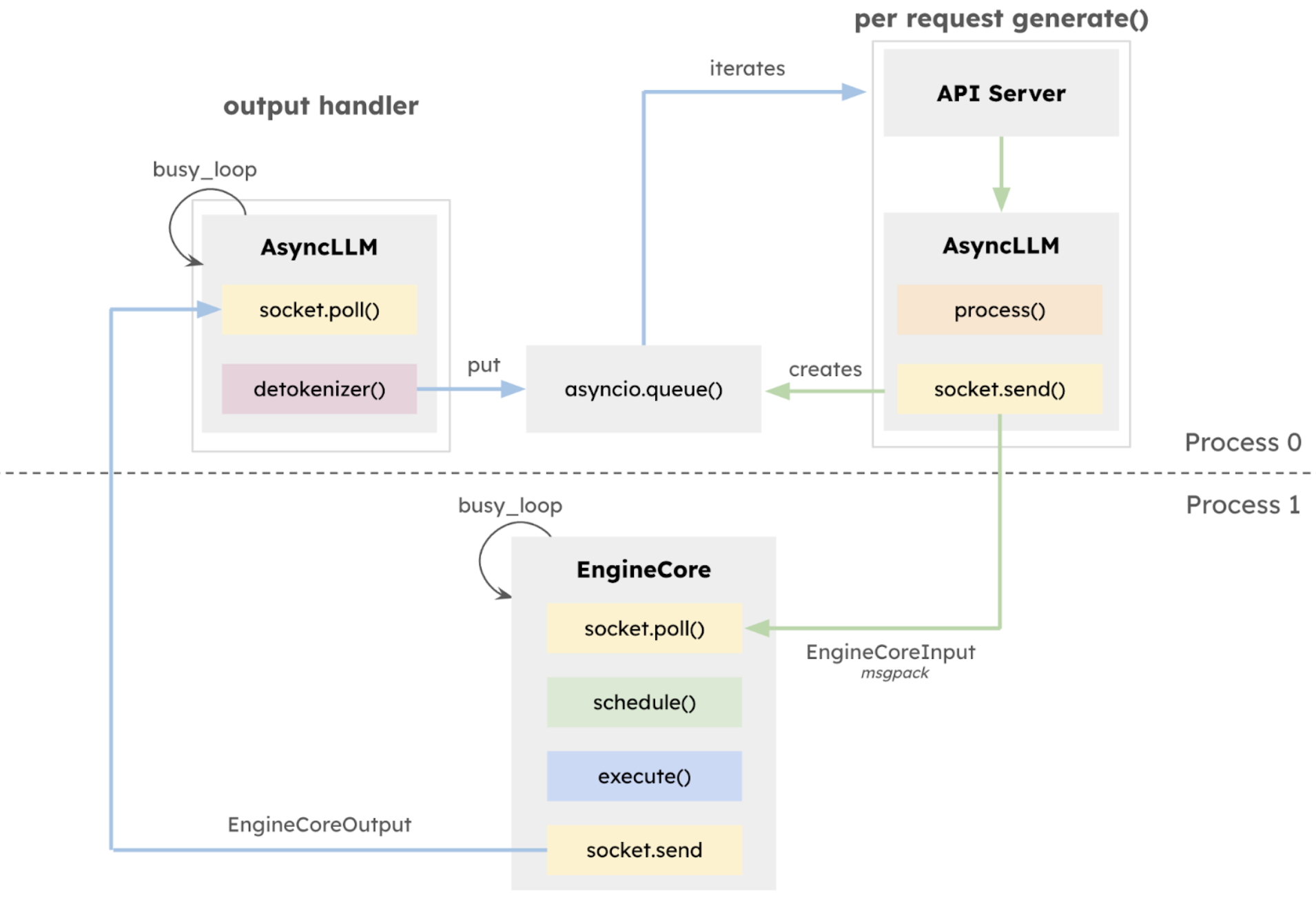
• Batch Scheduling Multiple Steps Ahead: This amortizes the CPU cost of scheduling over several GPU steps, keeping the GPU fed with work instead of waiting for the CPU.
• Asynchronous Output Processing: This overlaps the CPU work of handling model outputs (detokenization, stop condition checks) with the next GPU execution step.

These strategies are advanced, but they all stem from a single starting point: profiling the system to understand where the time is actually going.

Practical Profiling: Instrumenting Your API

Now, let's apply this principle to the FastAPI service you built in the last lesson. We will manually instrument our code to measure the time spent in each major stage of the request lifecycle. For production systems, you would use a dedicated library like OpenTelemetry, but building it from scratch provides a much deeper understanding.

We'll use Python's time.monotonic() for accurate duration measurement and a simple dictionary to store timestamps.

Here is the modified code from our previous lesson, now with detailed timing instrumentation:

import asyncio
import time
import random
from fastapi import FastAPI, Request, HTTPException, Response
from contextlib import asynccontextmanager
import logging




# --- Basic Configuration ---
logging.basicConfig(level=logging.INFO, format='%(asctime)s - %(message)s')
MAX_QUEUE_SIZE = 50




# --- Application State ---
app_state = {}

class TimingMiddleware:
    """
    A middleware to add timestamps to the start and end of a request.
    """
    async def __call__(self, request: Request, call_next):



        # Store initial timestamp in a request-specific state
        request.state.timings = {"request_received": time.monotonic()}
        
        response = await call_next(request)
        



        # After response is generated, add final timestamp and log
        request.state.timings["response_sent"] = time.monotonic()
        self.log_timings(request)
        
        return response

    def log_timings(self, request: Request):
        timings = request.state.timings
        if "processing_finished" not in timings: # e.g., for a 503 error
            total_duration = timings["response_sent"] - timings["request_received"]
            logging.info(f"REQUEST_REJECTED: Total duration: {total_duration*1000:.2f}ms")
            return




        # Calculate durations for each stage
        api_overhead = timings["entered_queue"] - timings["request_received"]
        queue_wait = timings["exited_queue"] - timings["entered_queue"]
        inference_time = timings["processing_finished"] - timings["exited_queue"]
        response_overhead = timings["response_sent"] - timings["processing_finished"]
        total_duration = timings["response_sent"] - timings["request_received"]

        log_message = (
            f"REQUEST_TIMING: "
            f"total={total_duration*1000:.2f}ms | "
            f"api_pre_queue={api_overhead*1000:.2f}ms | "
            f"queue_wait={queue_wait*1000:.2f}ms | "
            f"inference_work={inference_time*1000:.2f}ms | "
            f"api_post_inference={response_overhead*1000:.2f}ms"
        )
        logging.info(log_message)


async def inference_worker():
    """Simulates the inference engine worker."""
    logging.info("Inference worker started.")
    while True:
        try:
            request, timings = await app_state["request_queue"].get()
            
            timings["exited_queue"] = time.monotonic()
            
            processing_time = 0.1 # Simulate a fast GPU
            await asyncio.sleep(processing_time)
            
            timings["processing_finished"] = time.monotonic()




            # The response generation will happen back in the main thread for this example
            # In a real system, the worker might put the result in another queue.
            request['result_future'].set_result(timings)
            
            app_state["request_queue"].task_done()
        except asyncio.CancelledError:
            logging.info("Inference worker shutting down.")
            break

@asynccontextmanager
async def lifespan(app: FastAPI):
    """Manages application startup and shutdown."""
    logging.info("Application startup...")
    app_state["request_queue"] = asyncio.Queue(maxsize=MAX_QUEUE_SIZE)
    worker_task = asyncio.create_task(inference_worker())
    app_state["worker_task"] = worker_task
    yield
    logging.info("Application shutdown...")
    worker_task.cancel()
    await worker_task

app = FastAPI(lifespan=lifespan)
app.middleware("http")(TimingMiddleware())


@app.post("/predict")
async def predict(request: Request):
    """API endpoint that enqueues requests."""
    timings = request.state.timings
    
    try:



        # Mark time before attempting to enter queue
        timings["entered_queue"] = time.monotonic()
        



        # Create a future to wait for the result from the worker
        result_future = asyncio.Future()
        



        # Enqueue the request data along with the future
        request_item = {"data": await request.json(), "result_future": result_future}
        app_state["request_queue"].put_nowait((request_item, timings))
        



        # Wait for the worker to process this request and set the future's result
        final_timings = await result_future
        
        return Response(
            content='{"message": "Request processed successfully."}', 
            media_type="application/json"
        )

    except asyncio.QueueFull:
        logging.warning(f"Queue is full. Rejecting request. Queue size: {MAX_QUEUE_SIZE}")
        raise HTTPException(status_code=503, detail="Service Unavailable: Server is at capacity.")

Analysis of the Implementation

1. TimingMiddleware: This is a powerful FastAPI feature. It wraps every single request. We hook into it to record the request_received time at the beginning and the response_sent time at the very end. This gives us the true end-to-end duration.
2. request.state: This object is a property bag that lives for the duration of a single request. It's the perfect place to store our timings dictionary without polluting function signatures.
3. Timestamping Critical Points: We strategically place time.monotonic() calls at the boundaries of each logical stage:
   • Before put_nowait: entered_queue
   • After get() in the worker: exited_queue
   • After processing: processing_finished
4. asyncio.Future: This is a key change to enable accurate post-inference timing. The endpoint now waits on a Future that the worker resolves after processing is complete. This allows our middleware to correctly capture the time when the response is actually ready to be sent.

How to Test and Analyze

Run this code and use the same bash script from the previous lesson to generate a burst of traffic. Your logs will now contain detailed timing breakdowns for every request, like this:

REQUEST_TIMING: total=1015.43ms | api_pre_queue=0.15ms | queue_wait=1005.11ms | inference_work=100.12ms | api_post_inference=0.05ms
REQUEST_TIMING: total=915.20ms | api_pre_queue=0.18ms | queue_wait=904.78ms | inference_work=100.19ms | api_post_inference=0.05ms
REQUEST_REJECTED: Total duration: 0.89ms

From this output, you can immediately draw conclusions:

• The inference_work is consistently fast (~100ms), as we simulated.
• The queue_wait is enormous and is the dominant factor in total latency. This tells you the system is overloaded and requests are spending most of their life waiting.
• The api_pre_queue and api_post_inference overheads are negligible, meaning our FastAPI code is efficient. If these were high, it would point to a bottleneck in our Python API logic itself.
• Rejected requests are handled almost instantly (~1ms), confirming our load shedder is working efficiently.

This simple instrumentation gives you the power to diagnose performance issues with surgical precision.

Conclusion

You've now moved beyond treating the inference service as a black box. By instrumenting the end-to-end request path, you can precisely measure the latency contributed by each component—API handling, queuing, and model execution. This visibility is the non-negotiable first step toward targeted and effective optimization.

Key Takeaways:

• End-to-end latency is a sum of parts: To optimize the whole, you must measure the parts.
• CPU overhead is a real bottleneck: As demonstrated by vLLM, API servers, schedulers, and other CPU-bound logic can dominate latency, especially with fast GPUs and small models.
• Instrumentation is visibility: Simple, strategic timestamping can reveal where your system spends its time, distinguishing between queuing delays, processing time, and framework overhead.
• Profile, then optimize: The data from profiling tells you what to optimize. A long queue wait time suggests you need more workers or a faster model. High API overhead suggests you need to optimize Python code or even change the service architecture, as vLLM did.

Preview of the Next Lesson:
We have now built and profiled a sophisticated, robust API service on our local machine. The next logical step is to prepare it for the real world. In the next lesson, we will containerize the complete inference service and deploy it, packaging all the components and configurations you've built into a portable and scalable unit.