Choosing the Right Inference Mode: Batch, Asynchronous, Streaming, or Synchronous

Welcome back. In the last lesson, you translated an ML product prompt into sizing assumptions: peak request rate, candidate-score throughput, latency budgets, availability targets, data volumes, and an initial cost range. Those numbers now become selection criteria.

This lesson focuses on one architectural decision that interviewers often probe early: when and how should the model run? You will distinguish batch, asynchronous, streaming, and synchronous online inference, then choose among them using four requirements: required freshness, caller-facing latency, workload shape and scale, and total operational cost.

A useful caution at the outset: teams use asynchronous and streaming inconsistently. Do not win an interview by defending terminology. Win it by stating the execution contract precisely: What triggers scoring? Who, if anyone, waits? How fresh must the result be? Where is it stored or delivered?

---

Start with the contract, not the infrastructure

Before choosing Kafka, a feature store, GPUs, or a scheduler, establish four facts.

1. Freshness: How old may the input data or prediction be when it is used?
   “Fresh within a day” and “reflect a transaction within five seconds” lead to different designs.

2. Latency: Is a user or upstream service waiting? If so, what is the p95 or p99 deadline?
   A prediction needed before a checkout completes is fundamentally different from a score used in tomorrow’s email campaign.

3. Workload shape and scale: Are you scoring an entire population, individual submitted jobs, or an unbounded sequence of events? Is traffic steady, bursty, or periodic?

4. Cost and operational maturity: Can the business justify continuously running stream processors and highly available serving infrastructure? Or is high-throughput scheduled computation sufficient?

Keep freshness separate from latency:

• Freshness is the age or relevance of the information underlying a prediction.
• Latency is how long a caller waits after making a request.
• Throughput is how much work the system completes per unit time.

A precomputed recommendation can return in 5 ms from a key-value store but be 18 hours stale. Conversely, a stream processor can produce a score based on a just-arrived event without any end user waiting for it.

The following short video establishes the basic distinction between bounded batch work and continuously arriving stream work.

---

The four inference patterns

1. Batch inference: score a population on a schedule

With batch inference, a scheduler launches a job over a bounded dataset: perhaps all active users, products, accounts, or leads. The job reads data in bulk, scores many entities efficiently, and writes results to a warehouse, object store, or low-latency lookup store.

For example, a music service may generate recommendation candidates overnight for every recently active listener. When a listener opens the app, the API retrieves the latest stored candidates rather than executing the model at that moment.

Batch is a strong default when:

• predictions may be hours or days old;
• features change slowly;
• a large population must be scored regularly;
• scoring can exploit large, cost-efficient compute jobs;
• a simple, reliable first version matters more than real-time adaptation.

Its central limitation is staleness. If a job runs every $I$ hours and takes $T_{\text{run}}$ to complete, a conservative freshness bound is roughly:

$$S_{\text{max}}\approx I+T_{\text{run}}+T_{\text{source lag}}$$

The exact age depends on when the source snapshot is taken and when scores are published, but the interview point is simple: a daily batch cannot meet a requirement to react to behavior from the last minute.

Batch can also waste computation. If you rescore every registered user daily while only a small fraction visits, many predictions may never be used. That waste can still be acceptable when batch compute is inexpensive and the product value of fresh personalization is low.

2. Asynchronous inference: submit now, receive a result later

With asynchronous inference, a client submits a work item and receives an acknowledgement rather than waiting for the model result. A queue or job store buffers the request; workers score it later; the result is written to storage, sent through a callback, or made available for polling.

Typical examples include:

• extracting fields from a newly uploaded document;
• classifying a large image or video after upload;
• generating an account-risk report;
• performing an expensive enrichment step before a case reaches a human reviewer.

The contract is not “serve the answer within 100 ms.” It is “accept the job reliably, complete it within an agreed deadline, and make the result available.” That deadline may be seconds, minutes, or longer.

Asynchronous inference is useful when the work is too slow, expensive, or bursty for a request’s critical path, but needs to begin soon after submission. A queue gives the system backpressure and lets workers scale independently. The trade-off is that queue delay becomes part of the completion time:

$$T_{\text{completion}}=T_{\text{queue}}+T_{\text{feature work}}+T_{\text{inference}}+T_{\text{result delivery}}$$

An asynchronous design needs a plan for idempotency, retries, duplicate jobs, job status, and a dead-letter path for work that repeatedly fails. Those are not implementation footnotes; they are the operational contract.

Terminology note: some interview material calls scheduled bulk scoring “asynchronous batch inference.” That is reasonable because the caller is not waiting. In your answer, remove ambiguity: say either scheduled population batch scoring or per-request deferred job processing.

3. Streaming inference: score an event flow continuously

With streaming inference, an event triggers computation. Events such as transactions, clicks, device readings, delivery updates, or infrastructure metrics flow through a transport layer. A stream processor may maintain state and compute features, then a model scores each event or updated entity state. Outputs are written to another event stream, alerting system, or online store.

The defining properties are:

• the input is an ongoing, potentially unbounded event flow;
• no request caller waits for a direct response;
• freshness is often seconds or minutes rather than hours;
• stateful operations such as windows, counts, joins, and sessionization may be central.

Consider delivery-time estimation. A restaurant’s historical preparation time can be a batch feature, while the number of current orders and nearby driver supply change continuously. A streaming system can update these operational signals as events arrive, allowing downstream estimates to reflect current conditions.

Streaming is appropriate when:

• the product must react rapidly to events;
• the event itself is the natural trigger;
• predictions or features require continuously updated state;
• eventual output can be delivered asynchronously.

Its costs are not only compute costs. You operate event ingestion, ordering or partitioning behavior, state recovery, consumer lag monitoring, late-event handling, and replay procedures. Streaming can be efficient for stateful rolling calculations because it avoids repeatedly recomputing a large history in each batch. But it is usually not the cheapest way to process a one-time, massive historical backfill.

4. Synchronous online inference: return a prediction in the request path

With synchronous online inference, a client makes a request and waits while the system retrieves features, runs the model, and returns a prediction in the same request-response interaction.

This is the natural choice for:

• search ranking;
• a personalized feed assembled while a user waits;
• transaction fraud checks that must inform an authorization decision;
• content moderation required before publication;
• real-time eligibility or pricing decisions.

The serving path is a product dependency. Its p95 and p99 latency, availability, overload behavior, and fallback policy therefore matter as much as offline model quality.

A synchronous design can use current request context, such as a user’s query, location, cart contents, or most recent in-session activity. But “online” does not automatically mean that every feature is real-time. In practice, a low-latency request often combines:

• precomputed batch features;
• near-real-time features materialized by streaming;
• a small number of lightweight request-time features.

This limits the critical-path work. A complex database scan or broad aggregation at request time may produce fresh values but destroy tail latency under load.

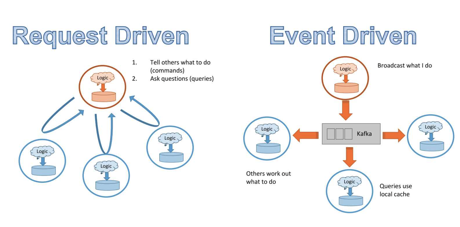
For a concise treatment of the patterns and their characteristic trade-offs, use the following reading.

---

Make the choice with a requirements matrix

The table below is a useful first-pass filter. Treat the ranges as design language, not universal hard limits.

Pattern	Trigger and consumer contract	Typical freshness target	Caller-facing latency	Cost and scale profile
Batch	Schedule triggers scoring of a bounded population; results are stored	Hours to days	Lookup can be low; model is off the request path	Excellent bulk efficiency; may score inactive entities unnecessarily
Asynchronous	A submitted job is queued; the submitter does not wait for the result	Usually current at processing time	Acknowledge quickly; completion may take seconds to minutes	Absorbs bursts and isolates costly work; needs queues, status, retries
Streaming	Each event or state update triggers continuous processing	Seconds to minutes	No direct caller wait	Good for continuous state and event scale; higher platform and operational complexity
Synchronous online	Request triggers scoring and the caller waits	Request-time context, subject to feature freshness	Usually tens to hundreds of milliseconds	Requires tail-latency headroom and high availability; scores only demanded traffic

Use this selection sequence in an interview:

1. Ask whether a caller is blocked.
   If yes, begin with synchronous online inference. You may later add a cached or batch fallback, but the immediate decision belongs in the request path.

2. If no caller waits, ask what triggers the work.
   A scheduled whole-population job suggests batch. A newly submitted document, image, or case suggests asynchronous job processing. A continuous transaction or sensor flow suggests streaming.

3. Turn freshness into a number.
   “Near real-time” is too vague. Ask whether it means 30 seconds, five minutes, or one hour. A five-minute requirement rules out a nightly batch, but it does not automatically require synchronous serving.

4. Check the economics at actual volume.
   Batch favors high-throughput bulk computation. Synchronous serving carries capacity headroom for peaks and tail latency. Streaming incurs persistent infrastructure and state-management costs. Async queues can smooth bursts but do not make expensive inference free.

5. Name the degradation mode.
   If synchronous scoring times out, should the system use cached results, a rules-based answer, a conservative decision, or a human-review path? If streaming falls behind, how stale can outputs become before they are withheld or replaced by a fallback?

---

One product often uses several patterns

A common weak interview answer is, “I would use streaming,” as though an entire ML system has one inference mode. The better answer assigns a pattern to each decision according to its contract.

Imagine a marketplace with recommendations, transaction risk, and seller-upload processing:

Product decision	Recommended pattern	Reason
Generate broad candidate lists for active shoppers	Batch	Long-term preferences and catalog signals can be refreshed periodically at low unit cost.
Update item popularity and shopper session features	Streaming	Clicks and purchases must affect features within seconds or minutes, without a user waiting on the stream processor.
Rank a shopper’s current candidate set	Synchronous online	The shopper is waiting for the page; current query and session context matter.
Analyze a seller’s uploaded product video	Asynchronous	The upload can be accepted immediately while expensive analysis completes in the background.
Decide whether to permit a payment	Synchronous online, with a fallback policy	The authorization flow needs a decision before it proceeds.

This composition resolves an apparent tension: streaming and synchronous online inference are often complements, not competitors. Streaming may keep features fresh; synchronous serving can read those materialized features within a strict request budget.

Similarly, batch scores can be a fallback for online ranking. If the real-time feature store or model server is unavailable, the service may return a precomputed candidate list. This lets the product maintain basic availability while clearly separating “usable experience” from “fully personalized experience.”

---

Cost reasoning without a false universal rule

There is no general rule that online or streaming inference is always more expensive than batch.

Batch usually has the best per-item compute efficiency because work is grouped into large jobs. But its total cost may be high if it repeatedly scores a huge inactive population.

Synchronous serving often avoids scoring inactive users because it scores on demand. Its cost comes from keeping capacity ready for peak traffic, multi-zone resilience, rapid autoscaling, feature lookups, and tail-latency headroom. Dynamic batching can improve accelerator utilization, but it introduces waiting time; it is a throughput optimization that must fit within the latency budget.

Streaming can avoid repeated recomputation of rolling state. For example, maintaining a 30-day engagement aggregate incrementally is often cheaper than scanning and recomputing the same 30-day history in frequent batch jobs. However, the operational cost of reliable stateful stream processing is real.

As a manager, phrase the trade-off in terms of product value:

“The decision is not whether real time is technically possible. It is whether the incremental business value of fresher predictions exceeds the added serving, streaming, and operational cost at projected scale.”

---

An interview-ready recommendation

A strong pattern-selection answer has five parts:

1. State the requirement.
   “The shopper is waiting for ranked results, with a 150 ms p95 endpoint budget, and recent session actions should affect ranking within a few seconds.”

2. Choose the primary serving mode.
   “I would use synchronous online inference for final ranking because the request cannot proceed without a result.”

3. Separate feature freshness from serving latency.
   “I would maintain session and popularity features through streaming, materialize them for fast reads, and avoid expensive aggregations in the request path.”

4. Use batch where it is economically appropriate.
   “I would precompute slower-changing embeddings and broad candidate sets in batch, then use them as inputs and fallbacks for online ranking.”

5. Name a fallback and a validation metric.
   “On online-serving degradation, return a cached or batch-generated list. I would validate the extra complexity through conversion lift from freshness, p95 latency, feature lag, and cost per thousand ranked requests.”

That structure shows that the inference pattern is a consequence of requirements, not a preferred technology stack.

---

Key takeaways

• Batch inference is scheduled bulk scoring: simple and efficient when hours or days of staleness are acceptable.
• Asynchronous inference accepts work now and produces a result later: useful for expensive or bursty per-item jobs that do not block a caller.
• Streaming inference reacts continuously to events and maintains fresh state: appropriate for event-driven outputs that need second- or minute-level freshness.
• Synchronous online inference belongs in the request path when a user or service must receive a prediction before proceeding.
• Separate freshness, caller latency, and throughput. They constrain one another, but they are not interchangeable.
• Most mature ML products combine patterns: batch for economical baseline computation, streaming for fresh features, and synchronous serving for user-facing decisions.
• In an interview, define the trigger, waiting party, freshness bound, output destination, fallback, and cost trade-off before naming infrastructure.

Next, you will design the data and feature layer that makes these choices reliable: validating data, preserving point-in-time correctness, tracking versions and lineage, and controlling access to features.