Introduction
Welcome to the first lesson of our new module on high-throughput serving. In the previous module, we focused on "static" optimizations—compressing the model with quantization and efficiently managing its memory with a paged KV cache. We squeezed as much performance as possible out of a single forward pass. However, a production inference server isn't processing one request; it's juggling hundreds or thousands. The next major frontier for optimization lies not in the model itself, but in how we schedule and process these concurrent requests.
This lesson tackles the most fundamental scheduling strategy: static batching. Your goal is to implement a conceptual model of static batching and, more importantly, to dissect and identify its profound inefficiencies when dealing with the variable-length inputs and outputs characteristic of LLM workloads. Understanding why this simple approach fails is the critical first step toward building high-performance serving systems.
1. The Rationale for Batching
Before we dive into how to batch, let's establish why it's essential. As you know from previous modules, the autoregressive decode phase consists of many forward passes, each generating a single token. Computationally, each step is dominated by matrix-vector multiplications.
On a powerful GPU, this is incredibly inefficient. The process is memory-bandwidth-bound: the GPU's powerful compute cores spend most of their time waiting for the model's weights to be loaded from High-Bandwidth Memory (HBM) for a very small amount of computation. GPU utilization during single-request decoding can be shockingly low, often under 5%.
Batching is the solution. By processing multiple requests simultaneously, we transform the memory-bound matrix-vector operations into more compute-bound matrix-matrix operations. The GPU loads the weights once per step and uses them for an entire batch of tokens, dramatically improving arithmetic intensity and overall hardware utilization.
LLM Serving from Scratch: The Systems Behind Fast Inference
The article 'LLM Serving from Scratch' provides an excellent explanation for why batching is so critical in the decode phase. This section sets the stage for our entire discussion on scheduling.
Please read the subsection titled '3.1 Why Batching Matters'. Focus on the explanation of how batching converts memory-bound operations into compute-bound ones, thereby improving GPU utilization.
2. Static Batching: The Simplest Approach
Static batching is the most straightforward way to implement batching. It mirrors the batching used during model training. The server follows a simple, rigid algorithm:
- Wait & Accumulate: The server waits for a certain number of requests to arrive (the batch size) or for a timeout to expire.
- Pad & Prefill: All requests in the batch are padded to the length of the longest input prompt. The server then runs one large prefill pass for the entire batch.
- Decode in Lockstep: The server performs decode iterations. In each iteration, every request in the batch generates one token.
- Wait for All to Finish: This is the critical step. The decoding process continues until the request generating the longest output sequence is complete.
- Return & Repeat: Once the last request is finished, the server returns all the results and is free to start processing the next batch.
To see this process explained, please watch the following segment.
Accelerating LLM Inference with vLLM
The 'Accelerating LLM Inference with vLLM' video from Databricks gives a very clear, concise overview of how static batching works and immediately hints at its primary inefficiency.
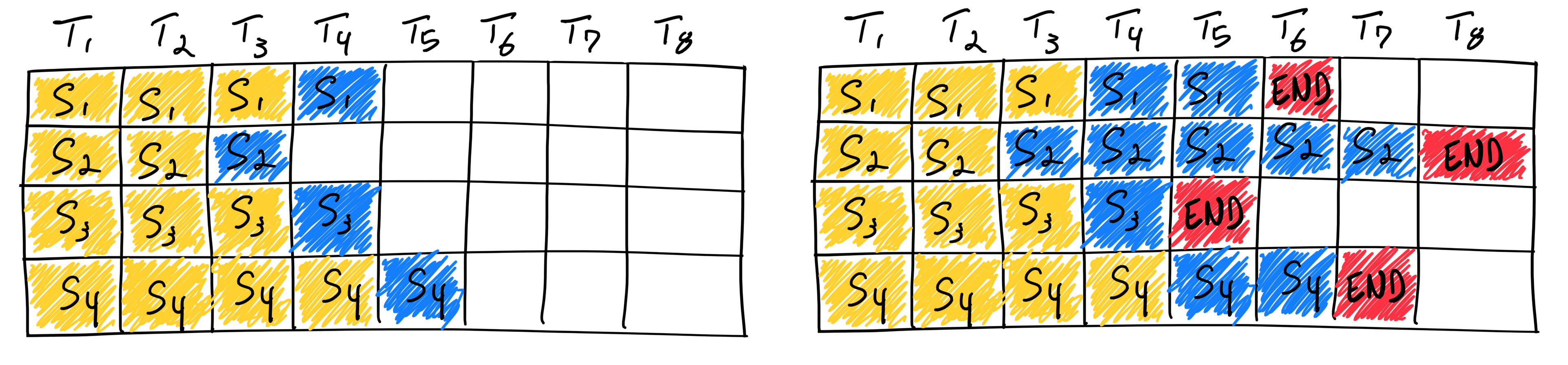
Watch the section from 00:19:26 to 00:21:12. Pay close attention to the animated diagram showing four sequences being processed and how some slots become idle (represented by white boxes) while waiting for the longest sequence.
3. Identifying the Core Inefficiency
The simplicity of static batching is also its fatal flaw. LLM inference workloads are characterized by high variability: prompts can be short or long, and requested outputs can range from a single word to thousands. Static batching is fundamentally unequipped to handle this variance efficiently.
The inefficiency manifests in several ways:
- Wasted Compute: When a short request in a batch finishes, its slot is not freed. For the remaining duration of the batch, the GPU continues to perform computations for that slot, processing padding tokens. This work is completely discarded, wasting valuable compute cycles.
- Wasted Memory: The KV cache for a completed request remains allocated in VRAM until the entire batch is finished. This memory could have been used to start processing a new, waiting request.
- Inflated Latency: A user who submits a simple request that should finish in milliseconds might have to wait seconds if it's batched with a request that requires a long, complex generation.
The diagram below perfectly illustrates this problem. Requests 3 and 1 finish early, but their compute slots are wasted for multiple time steps while they wait for the longer requests (especially request 2) to complete.
Let's quantify this waste.
LLM Serving from Scratch: The Systems Behind Fast Inference
The article 'LLM Serving from Scratch' provides a clear, numerical example of this computational waste.
Read the section '3.2 Static Batching (The Naive Approach)'. Focus on the calculation that shows how a batch with variable output lengths results in only 26% average GPU utilization. This quantifies the waste shown in the diagram above.
As the article demonstrates, the total computation performed is proportional to the batch size multiplied by the length of the longest sequence. The useful computation, however, is just the sum of the individual sequence lengths. This leads to the formal definition of static batching efficiency:
where is the batch size and is the output length of the i-th request.
You can see that if all are equal, efficiency is 100%. But as the variance in output lengths increases, the efficiency plummets.
4. A Practical Simulation of Static Batching
To make this tangible, let's turn to code. The following resource provides a Python simulation that models the behavior of static batching and calculates its efficiency. This serves as a conceptual implementation that isolates the scheduling logic from the complexities of a full inference pipeline.
Continuous Batching: Optimizing LLM Inference Throughput
This article, 'Continuous Batching', includes a simple yet powerful Python script to simulate and analyze static batching. It's a perfect hands-on exercise to solidify your understanding of the inefficiency.
First, read the section 'Static Batching' to understand the algorithm's five phases. Then, carefully study the Python code in the simulate_static_batch function and the subsequent analysis which shows a compute efficiency of only 53.8% for a sample workload. Make sure you understand how the wasted_iterations are calculated.
Let's review the core logic from the simulation:
# All requests must wait for the longest output
max_output = max(r.output_length for r in requests)


# Calculate wasted computation
total_iterations = len(requests) * max_output
useful_iterations = sum(r.output_length for r in requests)
wasted_iterations = total_iterations - useful_iterations

efficiency = useful_iterations / total_iterations
This simple block of code is the heart of the static batching problem. The total_iterations is dictated by the single max_output value, not the sum of useful work. Your task as a systems engineer is to close the gap between total_iterations and useful_iterations.
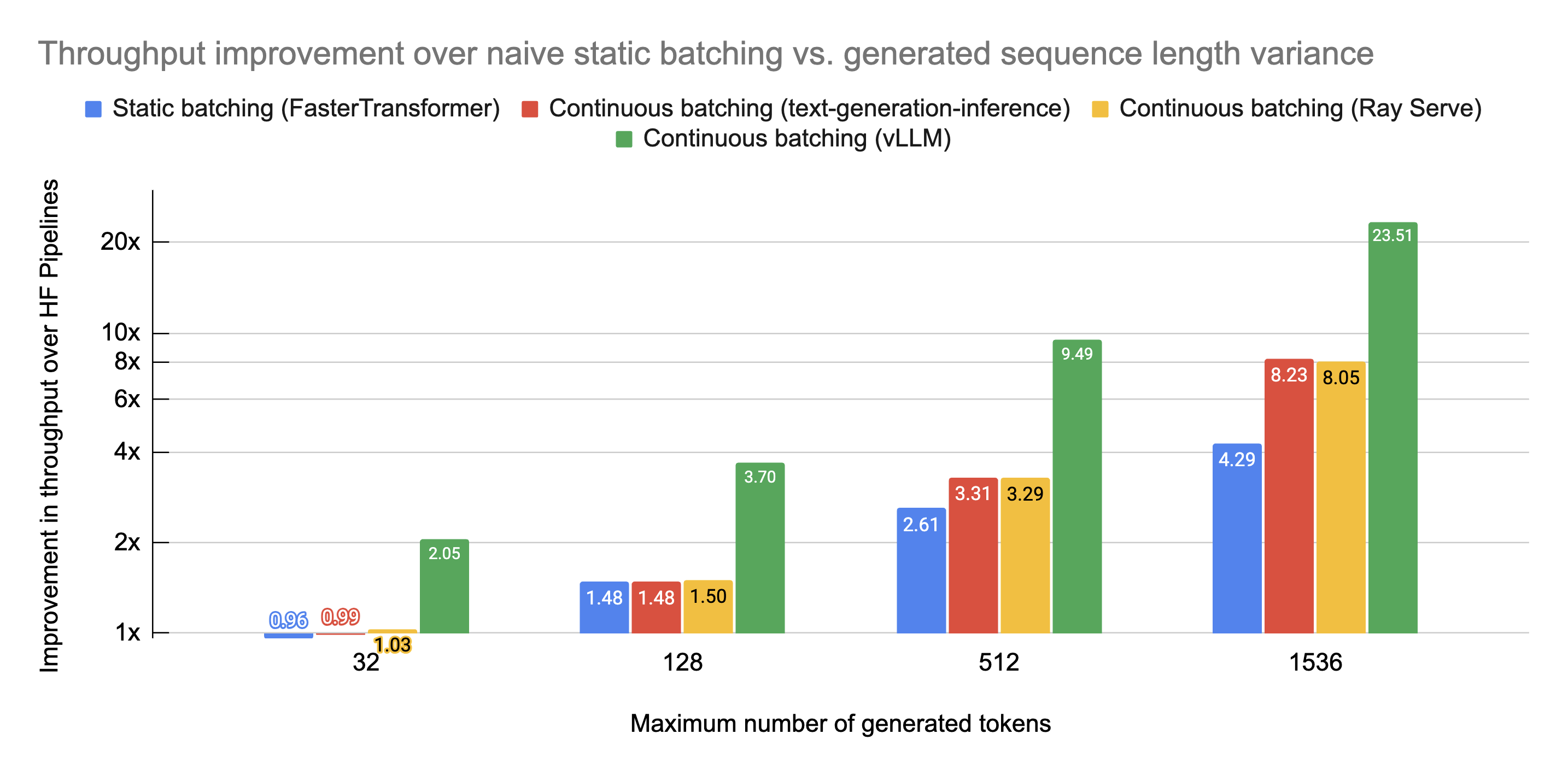
The consequences of this inefficiency are stark when comparing throughput against more advanced methods.
Conclusion
In this lesson, you have implemented a conceptual model of static batching and performed a detailed analysis of its shortcomings. While simple to implement, its rigid, lockstep nature is fundamentally mismatched with the dynamic and variable nature of LLM inference traffic.
Key Takeaways:
- Batching is necessary to overcome the memory-bandwidth bottleneck of the decode phase and achieve acceptable GPU utilization.
- Static batching is the naive approach, processing a fixed group of requests until all have completed.
- The primary inefficiency of static batching stems from variable input and output lengths, which lead to significant wasted compute and memory as finished requests idle in the batch.
- The latency of short requests is unfairly penalized, as they are forced to wait for the longest request in their batch to finish.
Preview of the Next Lesson:
The inefficiencies you've identified today directly motivate the need for a better solution. If the problem is that we are locked into a rigid batch, the solution must be to make the batch dynamic. In the next lesson, you will learn about and implement the core logic for continuous batching, a scheduling paradigm that operates at the iteration level to eliminate waste and dramatically increase throughput.