Fourier Transform for Sound Analysis

Welcome to the final lesson of our module on the physics of digital sound. In our last session, we explored the four basic waveforms, discovering that harmonically complex shapes like the sawtooth and square wave are actually built from a series of simple sine waves—a fundamental frequency plus a specific recipe of overtones. You now understand that a sound's timbre is defined by this harmonic content.

Today, we will formalize this concept by exploring the mathematical engine that allows us to deconstruct any complex sound into its constituent sinusoidal components. This tool is the Fourier transform. Our goal is for you to explain its role and understand intuitively how it works. For someone with your background in engineering and quantitative analysis, this concept serves as a bridge between the physical world of sound and the digital tools used to manipulate it. Understanding the Fourier transform is fundamental to grasping how equalizers, spectrum analyzers, and even certain types of synthesis truly operate.

The Two Worlds of Sound: Time and Frequency

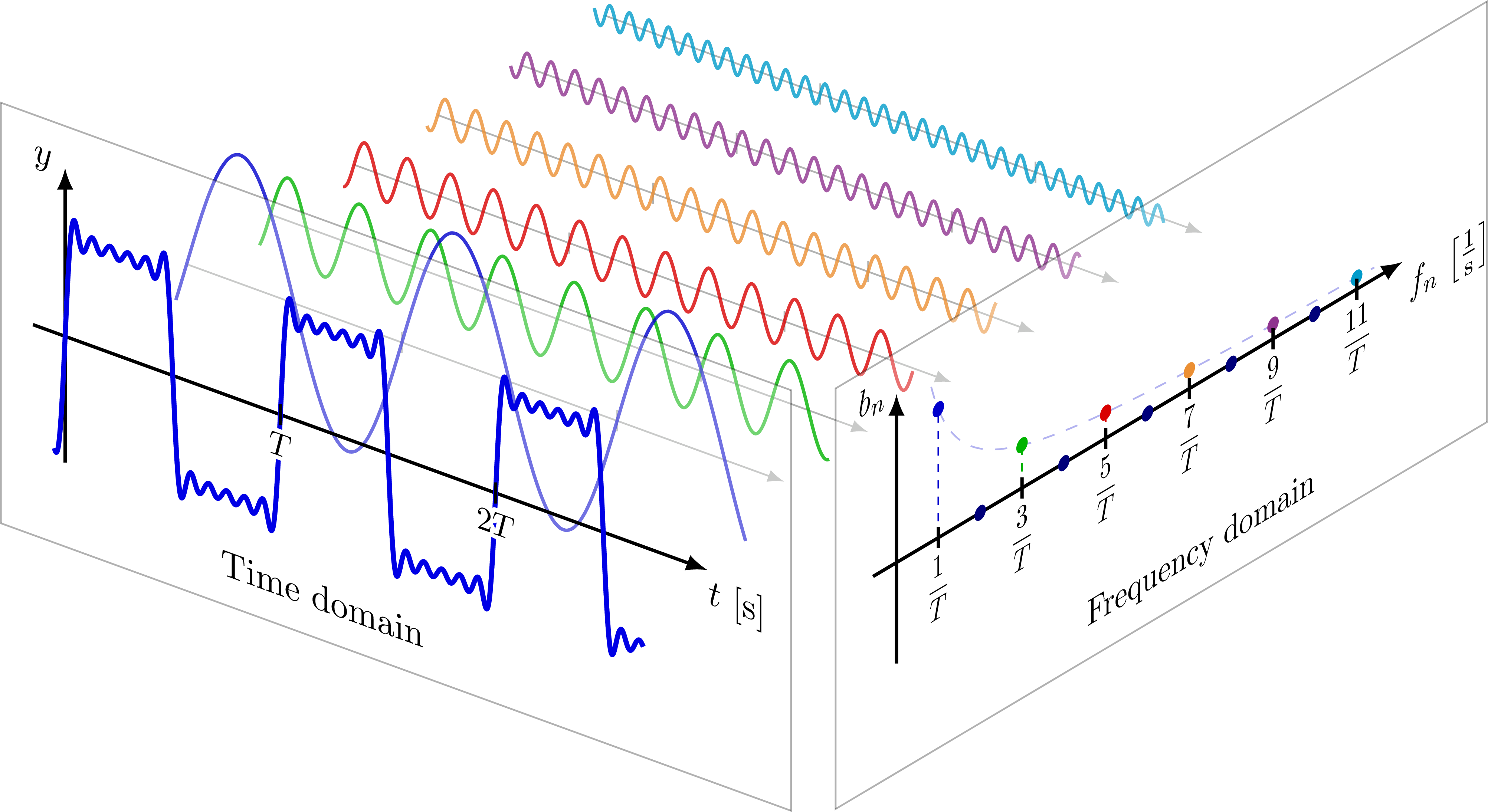
Every sound can be viewed from two different perspectives:

1. The Time Domain: This is the familiar waveform you see in an audio editor. It's a graph of pressure or amplitude versus time. It tells you the instantaneous level of the signal at any given moment.
2. The Frequency Domain: This is a graph of amplitude versus frequency. It doesn't show you the signal's moment-to-moment changes, but rather which frequencies are present in the signal over a period of time, and how strong they are. This is what you see on a spectrum analyzer.

The Fourier transform is the mathematical prism that allows us to move from the time domain to the frequency domain, breaking a complex signal down into its "spectral" components.

The process begins by recognizing that complex sounds are simply the sum of simpler ones. The following reading from the excellent 3Blue1Brown blog illustrates this fundamental starting point.

So, the central question is: given the final summed-up waveform, how do we find the original "recipe" of frequencies?

The Winding Machine: An Intuitive Look at the Transform

To understand how the Fourier transform isolates individual frequencies, we'll use a powerful visual analogy. Imagine taking your time-domain waveform and "wrapping" it around a circle. The speed at which you wrap it is a "test frequency" that you can control. The genius of the transform lies in what happens when your test frequency matches a frequency actually present in the signal.

The YouTube channel Sebastian Lague has created one of the best explanations of this process, building the concept from the ground up with code and visualizations. We'll walk through it step-by-step.

First, let's see how a complex signal is constructed, which recaps what we've learned and sets up the problem.

Now for the core idea. The video introduces the concept of plotting the signal around a circle and observing the "center of mass" of the resulting shape.

This is the key insight:

• When the test frequency does not match a frequency in the signal, the wound-up graph is balanced, and its center of mass stays at the origin (0,0).
• When the test frequency does match, the graph becomes lopsided, and the center of mass moves away from the origin.

Crucially, the position of this center of mass tells us everything we need to know about that frequency component:

• The distance from the origin is proportional to the amplitude of the frequency component.
• The angle tells us its phase.

Let's watch the next part where this is explicitly discussed.

Finally, to prove that this works, the video demonstrates the process in reverse: it takes a real audio signal, runs it through the Fourier transform to get the frequency data, and then reconstructs the original audio just from that data.

From Pictures to Mathematics

Your background allows us to peek under the hood and see how this "winding machine" is represented mathematically. The elegance of the formula lies in its use of complex numbers to describe the rotation.

The full formula for the Fourier Transform is:

$$\hat{g}(f)={\int }_{-\infty }^{\infty }g(t)e^{-2\pi ift}dt$$

This elegant expression encapsulates the entire process. For each frequency $f$ you want to test, you multiply your signal $g(t)$ by a rotating vector and integrate (average) over all time. The result, $\hat{g}(f)$, is a complex number whose magnitude is the amplitude and whose angle is the phase of that frequency component.

Practical Implementation: The Fast Fourier Transform (FFT)

In the real world of digital audio, we deal with discrete samples, not continuous functions. We also can't integrate to infinity. Instead, we use an algorithm called the Discrete Fourier Transform (DFT), and more commonly, its highly efficient version, the Fast Fourier Transform (FFT). This is what Ableton's Spectrum analyzer and EQs use.

The FFT works by analyzing short chunks of audio, or "blocks," one at a time. This introduces some important practical considerations.

The following reading from audio-measurement specialists NTi Audio provides a concise, professional overview of the practical aspects of the FFT.

Conclusion

In this lesson, we have lifted the lid on the Fourier transform, one of the most important concepts in digital signal processing. You now have a robust mental model for how complex sounds are deconstructed into simple sinusoidal components.

Here are the key takeaways:

• The Fourier transform is a mathematical tool that converts a signal from the time domain (waveform) to the frequency domain (spectrum).
• It works by "testing" for the presence of various frequencies, which can be visualized by wrapping the signal around a circle and observing its center of mass. The position of this center reveals the amplitude and phase of any matching frequency component.
• The formula $\hat{g}(f)=\int g(t)e^{-2\pi ift}dt$ is the mathematical expression of this "winding machine".
• In digital audio, we use the Fast Fourier Transform (FFT), which analyzes discrete blocks of audio and involves a crucial trade-off between time resolution and frequency resolution, determined by the block size.

This lesson concludes our module on the physics of digital sound. You've built a solid theoretical foundation, from the nature of digital audio and decibels to the harmonic content of waveforms and the transform that lets us analyze it.

Now it's time to put this theory into practice. In our next module, we will fire up Ableton Live. The first lesson will guide you through configuring its audio and MIDI preferences to ensure your system is set up for low-latency, professional-quality music production.