Bernoulli's Equation for Fluid Flow

Hello! Welcome to your next lesson in the Fluid Mechanics module.

In our last session, we explored the principle of conservation of mass, which gave us the continuity equation ($A_1{v}_1=A_2{v}_2$). This powerful tool allows us to determine how fluid velocity changes as the geometry of the flow path changes.

Today, we will build on that by introducing another fundamental conservation law: the conservation of energy. When applied to fluid flow, this leads us to one of the most famous and useful equations in all of engineering: Bernoulli's equation. This principle is the key to understanding how pressure, velocity, and elevation are interconnected in a moving fluid. For your goal of studying aerospace engineering, this equation is indispensable, as it forms the basis for understanding lift generation and measuring airspeed.

Your learning outcome for this lesson is to apply Bernoulli's equation to analyze pressure and velocity in frictionless fluid flow.

1. From Energy Conservation to Bernoulli's Equation

At its core, Bernoulli's equation is a simplified statement of the First Law of Thermodynamics applied to a moving fluid. It tells us that for an ideal fluid, the total energy along a streamline remains constant. This total energy has three components:

1. Flow Energy, related to pressure ($P$).
2. Kinetic Energy, related to velocity ($v$).
3. Potential Energy, related to elevation ($z$).

For an ideal, incompressible flow without any added work or heat, the energy conservation equation can be simplified directly into what we know as Bernoulli's equation. The following reading explains this transition without getting lost in a complex derivation, which aligns with your preference for a formula-based approach.

The resulting equation, in its most common "pressure" form, states that the sum of three pressure terms is constant between any two points (1 and 2) along a streamline:

$P_1+\frac{1}{2}\rho v_1^2+\rho g{z}_1=P_2+\frac{1}{2}\rho v_2^2+\rho g{z}_2$

Let's break down the terms:

• $P$ is the static pressure: This is the pressure you would measure if you were moving along with the fluid. It's the pressure exerted by the fluid in all directions at rest.
• $\frac{1}{2}\rho v^2$ is the dynamic pressure: This represents the kinetic energy of the fluid per unit volume. It's the pressure that arises from the fluid's motion.
• $\rho gz$ is the hydrostatic pressure: This represents the potential energy of the fluid per unit volume, due to its elevation $z$ in a gravitational field $g$.

The equation expresses a trade-off: if one term (like velocity) increases, another term (like pressure or elevation) must decrease to keep the total constant. This is the essence of many fluid phenomena.

2. The Three Forms of Bernoulli's Equation

Engineers use three common forms of Bernoulli's equation, which are all algebraically equivalent but have different units. Understanding these will be helpful, especially as we move into topics like energy losses.

To summarize the video:

1. Pressure Form: The one we've already seen. All terms have units of pressure (e.g., Pascals or N/m²).
   $P+\frac{1}{2}\rho v^2+\rho gz=\text{constant}$
2. Head Form: Divide the pressure form by $\rho g$. All terms now have units of length (e.g., meters). The term "head" refers to the equivalent height of a fluid column.
   $\frac{P}{\rho g}+\frac{v^2}{2g}+z=\text{constant}$
3. Energy Form: Divide the pressure form by $\rho$. All terms now have units of energy per unit mass (e.g., J/kg).
   $\frac{P}{\rho }+\frac{v^2}{2}+gz=\text{constant}$

For most problems in this lesson, we will use the pressure form, as it's often the most direct.

3. The Fine Print: Limitations of Bernoulli's Equation

Bernoulli's equation is powerful, but it's based on a set of strict assumptions about an "ideal" fluid. Applying it outside these conditions is one of the most common mistakes in fluid mechanics.

As the video explains, Bernoulli's equation is valid only when:

• The flow is steady (not changing with time).
• The fluid is incompressible ($\rho$ is constant).
• The flow is frictionless (inviscid). This means we ignore energy losses due to viscosity.
• The analysis is performed along a single streamline.
• There is no shaft work (no pumps or turbines) and no heat transfer between the two points of interest.

The "frictionless" assumption is the most significant limitation for real-world piping systems. As you saw in the video, friction causes a pressure drop that the simple Bernoulli equation cannot predict. We will address this in the next lesson by introducing the "Extended Bernoulli Equation".

4. Applications and Worked Examples

Now let's apply the equation to solve some classic engineering problems. In many cases, we will use Bernoulli's equation in tandem with the continuity equation you learned previously.

Application 1: The Venturi Meter

A Venturi meter is a device used to measure the flow rate in a pipe. It works by narrowing the pipe, which, according to the continuity equation, increases the fluid's velocity. Bernoulli's principle then tells us that this increase in velocity must be accompanied by a decrease in pressure. By measuring this pressure difference, we can calculate the flow rate.

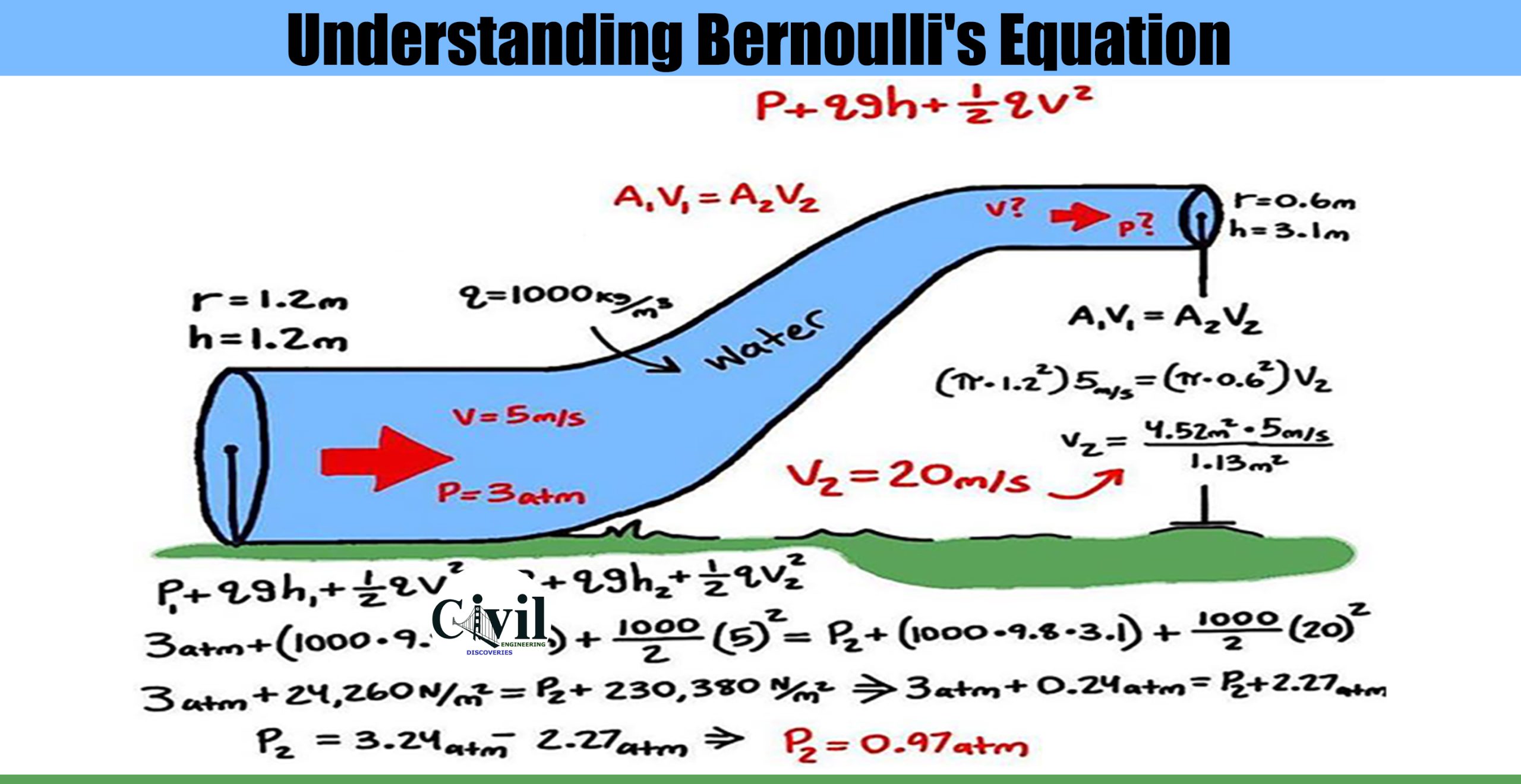
Let's watch a detailed walkthrough of a Venturi tube problem.

Test your understanding!

Water ($\rho =1000{\text{ kg/m}}^3$) flows through a horizontal pipe. At point 1, the diameter is 10 cm and the pressure is 200 kPa. At point 2, the pipe narrows to a diameter of 5 cm. If the velocity at point 1 is 2 m/s, what is the pressure at point 2? (Assume frictionless flow).

Show answer

1. Find the velocity at point 2 using the continuity equation.

   • $A_1=\frac{\pi (0.1\text{ m}{)}^2}{4}=0.0025\pi {\text{ m}}^2$
   • $A_2=\frac{\pi (0.05\text{ m}{)}^2}{4}=0.000625\pi {\text{ m}}^2$
   • From $A_1{v}_1=A_2{v}_2$, we get $v_2=v_1\frac{A_1}{A_2}=(2\text{ m/s})\frac{0.0025\pi }{0.000625\pi }=2\times 4=8\text{ m/s}$.

2. Apply Bernoulli's equation.

   • Since the pipe is horizontal, the elevation term $z$ is constant ($z_1=z_2$), so $\rho gz$ cancels from both sides.
   • $P_1+\frac{1}{2}\rho v_1^2=P_2+\frac{1}{2}\rho v_2^2$
   • Solve for $P_2$: $P_2=P_1+\frac{1}{2}\rho (v_1^2-v_2^2)$

3. Substitute the values.

   • $P_2=200,000\text{ Pa}+\frac{1}{2}(1000{\text{ kg/m}}^3)((2\text{ m/s}{)}^2-(8\text{ m/s}{)}^2)$
   • $P_2=200,000+500(4-64)$
   • $P_2=200,000-30,000=170,000\text{ Pa}=170\text{ kPa}$.

Application 2: Lift and Airspeed in Aerospace

Bernoulli's principle is fundamental to aerodynamics.

• Lift on an Airfoil: An aircraft wing (airfoil) is shaped to make air travel faster over its curved top surface than its flatter bottom surface. According to Bernoulli, this higher velocity on top creates a lower pressure zone, while the lower velocity below creates a higher pressure zone. This pressure difference results in a net upward force called lift.

• Measuring Airspeed with a Pitot-Static Tube: This is a crucial instrument on every aircraft.

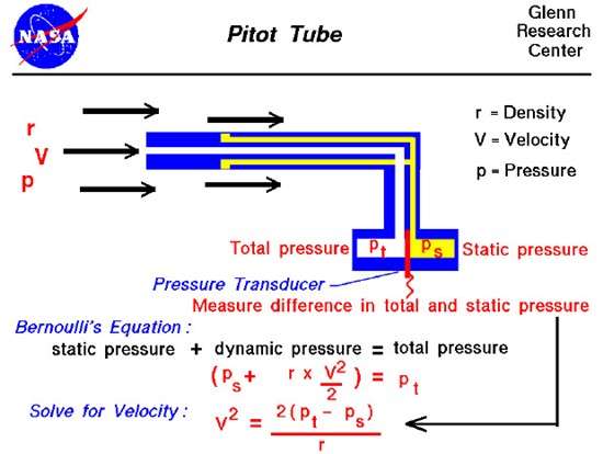
Let's apply Bernoulli's equation to the Pitot tube. Let point 1 be the stagnation point ($v_1=0$) and point 2 be a point in the undisturbed airflow ($v_2=v_{airspeed}$). Both points are at the same altitude ($z_1=z_2$).

$P_{stagnation}+\frac{1}{2}\rho (0{)}^2=P_{static}+\frac{1}{2}\rho v_{airspeed}^2$

Rearranging to solve for the airspeed gives the famous Pitot formula:
$v_{airspeed}=\sqrt{\frac{2(P_{stagnation}-P_{static})}{\rho }}$

The term $P_{stagnation}-P_{static}$ is exactly the dynamic pressure, which is what the instrument measures.

Conclusion

Today, we've unlocked one of the most important relationships in fluid mechanics. By applying the principle of energy conservation, we derived Bernoulli's equation, which connects a fluid's pressure, velocity, and elevation.

Key Takeaways:

• Bernoulli's Equation is a statement of energy conservation for an ideal fluid flow: $P_1+\frac{1}{2}\rho v_1^2+\rho g{z}_1=P_2+\frac{1}{2}\rho v_2^2+\rho g{z}_2$.
• It represents a balance between static pressure, dynamic pressure, and hydrostatic pressure.
• The equation is only valid for steady, incompressible, frictionless flow with no work or heat transfer.
• In practice, it is used with the continuity equation to solve problems where both area and pressure/elevation change.
• It provides the fundamental explanation for lift generation on an airfoil and is used directly to calculate airspeed with a Pitot-static tube.

Next Steps:
We've established the ideal case. However, as we saw, real-world flows always involve friction, which results in a loss of energy (or "head"). In our next lesson, we will tackle this by introducing the Extended Bernoulli Equation. We will learn how to quantify frictional losses in pipes using the Darcy-Weisbach equation and the Moody chart, making our analyses much more realistic.