FM: Math and Bandwidth

Hello! Welcome back to our course on radioelectronics.

In our last few lessons, we've focused on Amplitude Modulation (AM), where information is encoded by varying the amplitude of a carrier wave. We saw how this leads to a relatively simple spectrum and allows for straightforward demodulation using an envelope detector.

Today, we shift our focus to a different and widely used modulation scheme: Frequency Modulation (FM). Instead of altering the carrier's amplitude, FM encodes information by varying its instantaneous frequency. This lesson will cover the mathematical principles behind FM and the methods used to estimate its bandwidth, which is a critical parameter for any communication system.

1. The Mathematical Representation of an FM Wave

The fundamental principle of FM is that the instantaneous frequency of the carrier signal, $f_{i} (t)$ , deviates from its resting frequency, $f_{c}$ , in direct proportion to the amplitude of the message signal, $m (t)$ .

This relationship is expressed as:
$f_{i} (t) = f_{c} + k_{f} m (t)$
where $k_{f}$ is the frequency sensitivity of the modulator, with units of Hz/Volt. This constant determines how much the carrier frequency changes for a given message signal amplitude.

To derive the full expression for the FM wave, we need to relate frequency to phase. Recall that the instantaneous angular frequency $ω_{i} (t)$ is the time derivative of the total phase angle $θ_{i} (t)$ :
$ω_{i} (t) = \frac{d θ _{i} ( t )}{d t}$
Since $ω_{i} (t) = 2 π f_{i} (t)$ , we can find the phase by integrating the instantaneous frequency over time.

Mathematical representaion of FM

The following resource provides a clear, step-by-step derivation of the general mathematical expression for an FM wave. It's a foundational piece of theory for this topic.

Please read the first three pages of this document, from the beginning down to the section titled 'Single-tone FM'. Focus on how the definition of instantaneous frequency, f_i = f_c + k_f m(t), is integrated to determine the phase angle heta_i and ultimately leads to the general expression for an FM wave.

As you've just read, by integrating the expression for the instantaneous angular frequency, we arrive at the general form of an FM signal:
$s_{FM} (t) = A_{c} cos (θ_{i} (t)) = A_{c} cos (2 π f_{c} t + 2 π k_{f} \int_{0}^{t} m (τ) d τ)$
Notice two key characteristics:

The amplitude $A_{c}$ is constant, unlike in AM.
The message signal $m (t)$ is embedded within the phase of the carrier through integration. This non-linear relationship is what makes the analysis of FM more complex than AM.

Single-Tone Modulation

For analysis, it's common to consider a simple sinusoidal message signal, $m (t) = A_{m} cos (2 π f_{m} t)$ . Substituting this into the general FM equation and performing the integration yields a more specific and very important form of the FM wave.

Mathematical representaion of FM

Now, let's examine the specific case of single-tone modulation and define the key parameters that characterize an FM signal.

Please read the sections 'Single-tone FM', 'FREQUENCY DEVIATION', and 'MODULATION INDEX' (pages 3-5). Pay close attention to how the general FM equation simplifies for a sinusoidal message and how the terms for frequency deviation (\Delta f) and modulation index (m_f) are defined.

From this reading, we can define the essential parameters for single-tone FM:

Frequency Deviation ( $Δ f$ ): This is the maximum frequency shift from the carrier frequency $f_{c}$ . It is directly proportional to the amplitude of the message signal, $A_{m}$ .
$Δ f = k_{f} A_{m}$
In audio terms, $Δ f$ corresponds to the loudness of the modulating signal. For commercial FM radio in the 88-108 MHz band, the maximum allowed frequency deviation is 75 kHz.
Modulation Index ( $β$ or $m_{f}$ ): This is a dimensionless ratio that compares the frequency deviation to the modulating frequency.
$β = \frac{Δ f}{f _{m}}$
The modulation index is crucial as it determines the spectral characteristics of the FM signal.

With these definitions, the equation for a single-tone FM wave becomes:
$s_{FM} (t) = A_{c} cos (2 π f_{c} t + β sin (2 π f_{m} t))$

2. The FM Spectrum and Bandwidth Estimation

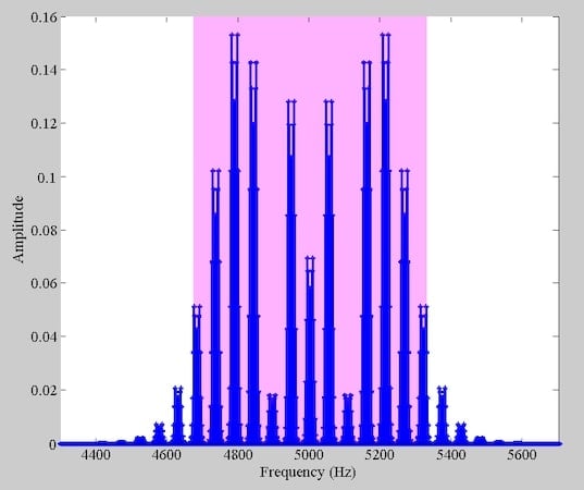
Unlike AM, where modulation creates just two sidebands, the non-linear nature of FM generates a theoretically infinite number of sidebands at frequencies $f_{c} \pm n f_{m}$ , where $n$ is any integer.

The amplitudes of these sidebands are described by Bessel functions of the first kind, denoted $J_{n} (β)$ . The amplitude of the sideband at $f_{c} \pm n f_{m}$ is proportional to $J_{n} (β)$ . While we won't delve into solving Bessel functions, it's important to recognize their role in defining the FM spectrum.

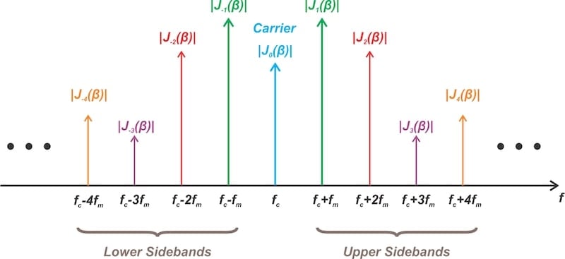
This spectrum plot illustrates the components of an FM signal. The central line is the carrier at frequency $f_c$ with amplitude proportional to $J_0(\beta)$. It is surrounded by pairs of sidebands at $f_c \pm f_m$, $f_c \pm 2f_m$, etc., with amplitudes determined by $J_1(\beta)$, $J_2(\beta)$, and so on.

The amplitudes of the sidebands depend entirely on the modulation index $β$ .

Frequency Modulation, FM Sidebands & Bandwidth

This resource provides a good conceptual overview of FM sidebands and introduces a famous rule of thumb for estimating bandwidth.

Please read the section 'Frequency modulation sidebands' and look at the table of relative sideband amplitudes. Note how the carrier and sideband amplitudes change with the modulation index. Then, briefly read the section 'Equations & calculation for FM sideband levels' to appreciate the complexity that justifies using an approximation for bandwidth.

As you saw, for certain values of $β$ , the carrier component $J_{0} (β)$ can even go to zero, meaning all the signal power is in the sidebands.

Carson's Rule for Bandwidth Estimation

Since the spectrum is theoretically infinite, we need a practical way to define the bandwidth that contains most of the signal's power (typically 98-99%). The most widely accepted approximation is Carson's Rule.

Carson's Rule states that the bandwidth (BW) of an FM signal is approximately twice the sum of the maximum frequency deviation and the highest modulating frequency.

$B W \approx 2 (Δ f + f_{m})$

This plot shows an FM spectrum with the bandwidth estimated by Carson's Rule highlighted. While some sidebands exist outside this region, their power is considered negligible for most practical purposes.

This rule elegantly combines the two factors that spread the signal's energy: the deviation ( $Δ f$ ) and the modulating frequency ( $f_{m}$ ).

Frequency Modulation, FM Sidebands & Bandwidth

Let's look at the formal statement of Carson's Rule and how it's applied.

Read the section 'Carson's Rule for FM bandwidth'. Pay attention to the formula and the example given for a typical broadcast FM signal.

A classic example is commercial FM broadcasting:

Maximum frequency deviation, $Δ f = 75$ kHz.
Maximum audio modulating frequency, $f_{m} = 15$ kHz.

Applying Carson's Rule:
$B W \approx 2 (75 kHz + 15 kHz) = 2 (90 kHz) = 180 kHz$
This is why commercial FM stations are allocated channel bandwidths of 200 kHz, providing a small guard band.

Carson's rule also helps distinguish between two types of FM:

Narrowband FM (NBFM): When $β ≪ 1$ , $Δ f$ is much smaller than $f_{m}$ . Carson's rule simplifies to $B W \approx 2 f_{m}$ , which is the same bandwidth as an AM signal.
Wideband FM (WBFM): When $β ≫ 1$ , $Δ f$ is much larger than $f_{m}$ . Carson's rule simplifies to $B W \approx 2Δ f$ . This is the case for high-fidelity FM broadcasting.

3. Practice Problem

Let's apply these concepts. Consider an FM signal represented by the voltage equation:
$v (t) = 12 cos (2 π \cdot 95 \cdot 1 0^{6} t + 5 sin (2 π \cdot 20 \cdot 1 0^{3} t))$
Let's determine its key parameters.

By comparing this to the standard form $s_{FM} (t) = A_{c} cos (2 π f_{c} t + β sin (2 π f_{m} t))$ , we can identify:

Carrier Frequency ( $f_{c}$ ): $f_{c} = 95 \cdot 1 0^{6}$ Hz = 95 MHz
Modulating Frequency ( $f_{m}$ ): $f_{m} = 20 \cdot 1 0^{3}$ Hz = 20 kHz
Modulation Index ( $β$ ): $β = 5$
Frequency Deviation ( $Δ f$ ): We know $β = Δ f / f_{m}$ , so:
$Δ f = β \cdot f_{m} = 5 \cdot 20 kHz = 100 kHz$
Carson's Rule Bandwidth (BW):
$B W \approx 2 (Δ f + f_{m}) = 2 (100 kHz + 20 kHz) = 2 (120 kHz) = 240 kHz$

Conclusion

In this lesson, we have established the fundamental principles of Frequency Modulation. We derived its mathematical representation and saw how it differs significantly from AM, particularly in its non-linear nature and spectral complexity.

Key Takeaways:

In FM, the instantaneous frequency of a carrier wave is varied in proportion to the message signal's amplitude: $f_{i} (t) = f_{c} + k_{f} m (t)$ .
The resulting FM wave has a constant amplitude, with the information encoded in the phase term: $s_{FM} (t) = A_{c} cos (2 π f_{c} t + 2 π k_{f} \int m (t) d t)$ .
For a single-tone modulating signal, the key parameters are the frequency deviation ( $Δ f$ ), which is proportional to the message amplitude, and the modulation index ( $β = Δ f / f_{m}$ ).
The spectrum of an FM signal consists of a carrier and theoretically infinite sidebands, with amplitudes determined by Bessel functions of the modulation index $β$ .
Carson's Rule, $B W \approx 2 (Δ f + f_{m})$ , provides a robust and widely used estimate for the practical bandwidth of an FM signal.

Now that you understand how an FM signal is mathematically described and how its bandwidth is characterized, the next logical step is to learn how to recover the original message signal. In our next lesson, we will explore FM Demodulation, focusing on techniques such as the slope detector and the more advanced Phase-Locked Loop (PLL).