Analyzing Self-Supervised Speech Representations

Hello! Welcome to the final lesson of our module on self-supervised speech representation.

In our last lesson, we established that self-supervised models are powerful because they learn universal representations that enable transfer learning across many languages and downstream tasks. We saw that a single pre-trained model can be the foundation for ASR, speaker identification, and even generative audio systems.

This naturally leads to a crucial question: if these representations are so powerful, what exactly do they contain? Today, we will move from observing the effects of these representations to investigating their content. Our goal is to answer the learning outcome: Explore and analyze the learned representations from a self-supervised speech model.

We will "peek inside the black box" to understand what kind of information is encoded at different layers of a model like wav2vec 2.0 or HuBERT. This is a critical skill for a researcher, as understanding a model's internal workings can lead to better model design, more effective fine-tuning strategies, and novel applications.

By the end of this lesson, you will understand:

• The primary methods for analyzing neural representations: probing and direct correlation analysis.
• The concepts of Canonical Correlation Analysis (CCA) and Mutual Information (MI) as tools for this analysis.
• The typical hierarchical structure of information in a speech model, from acoustic to phonetic to lexical content.
• How to use a practical toolkit like S3PRL to extract representations for your own analysis.

1. The Art of "Model-ology": How to Analyze Representations

When we say we want to "analyze a representation," we're asking a specific question: for a given layer in a neural network, does its output vector (the representation) contain meaningful, predictable information about a specific property of the input? These properties could be:

• Acoustic: Speaker identity, pitch, energy.
• Phonetic: The phoneme being spoken at that moment.
• Lexical: The word identity.
• Semantic: The meaning of the word or utterance.

There are two main families of techniques to answer this question.

Method 1: Probing Classifiers

The most intuitive method is called probing. The idea is simple: if a layer's representation truly contains information about a property (like phonemes), then a simple classifier should be able to predict that property from the representation.

Let's watch a video that introduces this concept clearly.

The process for probing a speech model is as follows:

1. Freeze the pre-trained model (e.g., wav2vec 2.0).
2. Extract hidden-state vectors from a specific layer for a dataset with known labels (e.g., phoneme labels from a forced-aligned corpus).
3. Train a simple probe (e.g., a linear classifier) to map the hidden-state vectors to their corresponding labels.
4. Evaluate the probe's accuracy. A high accuracy suggests that the chosen layer encodes the target property well. By repeating this for every layer, you can map out where in the model different types of information are most prominent.

Method 2: Direct Correlation Analysis

A second approach avoids training an additional model. Instead, it uses statistical measures to directly quantify the relationship between the model's representations and vectors that represent the properties of interest. The paper "Layer-wise analysis of a self-supervised speech representation" uses two key methods.

As described in the paper, the two main tools are:

• Canonical Correlation Analysis (CCA): This method measures the linear correlation between two sets of multidimensional vectors. It's used to compare the model's representations (continuous vectors) with other continuous representations of a property. For example, to check for acoustic information, you could measure the CCA between a layer's output and MFCC features. To check for semantic information, you could measure the CCA between a layer's output and GloVe word embeddings. A high CCA score indicates that the information in one vector space can be linearly transformed into the other, suggesting they encode similar information.

• Mutual Information (MI): This method measures how much information the presence of one variable reveals about another. It is ideal for comparing the model's continuous representations with discrete properties like phoneme or word IDs. To do this, the continuous representation vectors are first clustered (using an algorithm like K-means) to produce discrete cluster IDs. Then, MI is calculated between these cluster IDs and the ground-truth labels (e.g., phoneme IDs). High MI indicates a strong dependency, meaning the layer's representation effectively separates different phonemes or words. This process of clustering continuous speech into discrete units should remind you of the HuBERT pre-training strategy.

2. Case Study: What's Inside wav2vec 2.0?

Now that we understand the methods, let's look at the results. What do these analyses reveal about a model like wav2vec 2.0? The paper by Pasad et al. provides a fantastic summary of findings.

The analysis reveals several fascinating patterns:

1. Linguistic Hierarchy: The model learns representations that follow the natural hierarchy of speech processing.

   • Shallow layers (close to the input) are best at encoding low-level acoustic features. They show high correlation with mel spectrograms.
   • Mid-layers become specialized for phonetic information. Probes trained on these layers are best at predicting phoneme labels.
   • Deeper layers start capturing word-level information. They show higher MI with word labels and higher CCA with semantic word embeddings like GloVe.

2. Autoencoder-like Behavior: The paper notes an "autoencoder-style behaviour." The representations in the early layers are very similar to the input features. They diverge in the middle layers to capture more abstract linguistic content, and then, surprisingly, the final layers start to resemble the input features again, as if trying to reconstruct the original signal.

3. Impact of Fine-tuning: When the model is fine-tuned for ASR, this pattern changes. The later layers, in particular, stop trying to reconstruct the input and become highly specialized for predicting characters or words, breaking the autoencoder-like symmetry. This insight led the authors to a practical discovery: re-initializing the final two layers before fine-tuning actually improved ASR performance, as these layers were not optimally pre-trained for the ASR task.

This demonstrates that analyzing representations is not just an academic exercise—it provides concrete insights that can improve model performance.

3. A Brief Look Inside HuBERT

The same principles apply to other models like HuBERT. Recall from previous lessons that HuBERT's pre-training involves predicting discrete "hidden units" that are generated by clustering audio features. This is a form of representation learning itself.

The "hidden units" that HuBERT learns are themselves a rich, discretized representation of speech. Probing and analyzing the Transformer layers that process these units would reveal a similar hierarchical structure to the one found in wav2vec 2.0.

4. Practical Steps: Extracting Representations with S3PRL

Theory is great, but as a developer and researcher, you need to know how to get your hands on these representations. A fantastic tool for this is the S3PRL (Self-Supervised Speech Pre-training and Representation Learning) Toolkit.

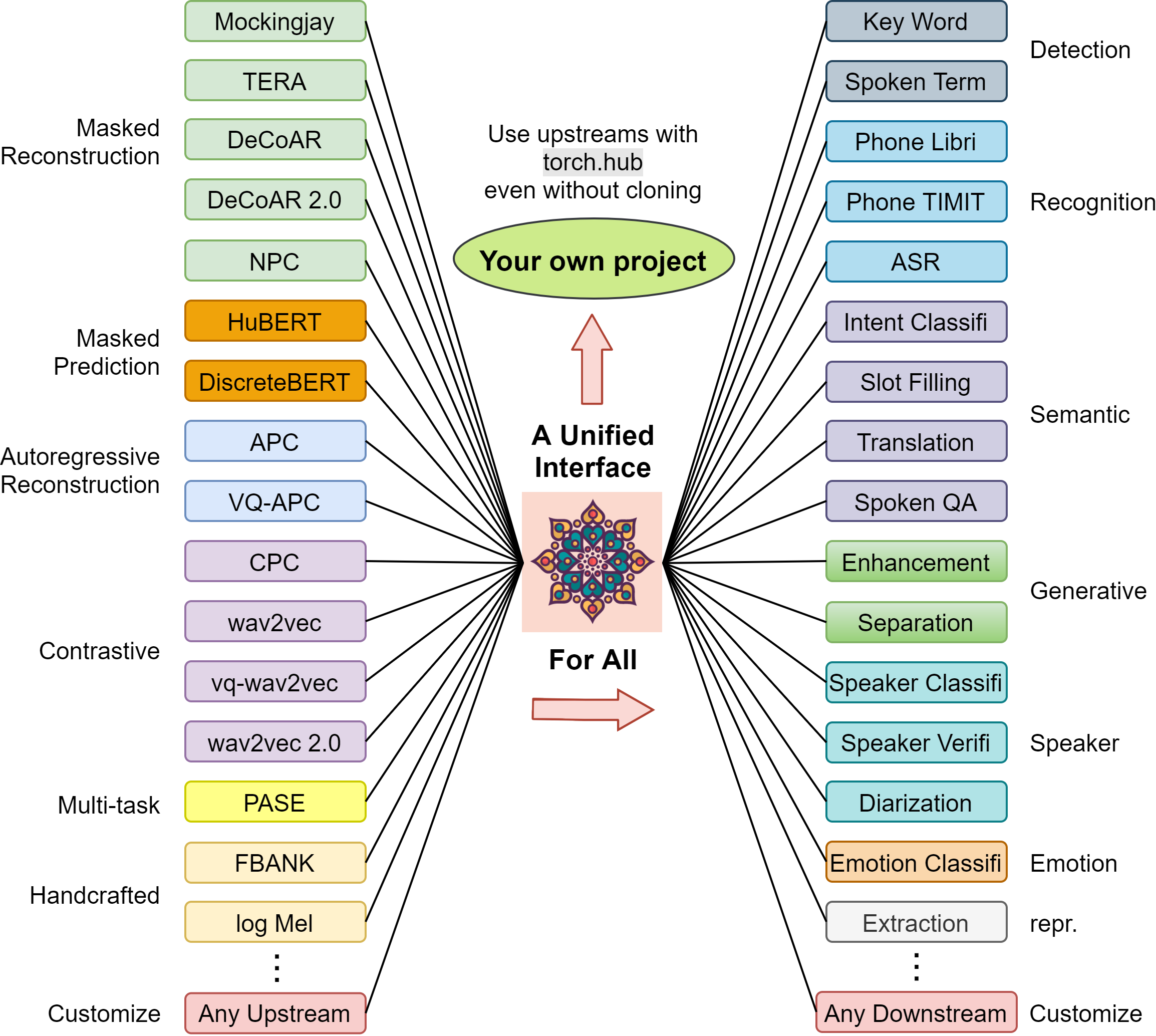
S3PRL, which is integrated with the ESPnet toolkit you're interested in, allows you to easily load almost any major pre-trained speech model and extract its hidden states.

Here is the core idea from the documentation, presented as a standalone code block. This is the starting point for any analysis:

# 1. Install the S3PRL package
# pip install s3prl

import torch
from s3prl.nn import S3PRLUpstream




# 2. Load a pre-trained model (e.g., HuBERT base) with one line
# The model is automatically downloaded from torch.hub
model = S3PRLUpstream("hubert")
model.eval()




# 3. Create a dummy audio input
# Batch of 2 waveforms, each 2 seconds long (at 16kHz)
wavs = [torch.randn(16000 * 2), torch.randn(16000 * 1)]




# 4. Extract all hidden states from the model
with torch.no_grad():



    # The model returns a list of tensors, one for each layer's hidden states
    all_hidden_states, hidden_states_lengths = model(wavs)




# 5. Inspect the output
print(f"Number of layers (including input embeddings): {len(all_hidden_states)}")



# HuBERT base has 13 hidden states: 1 for input embeddings + 12 for Transformer layers
# Output shape: (batch_size, sequence_length, hidden_dimension)
print(f"Shape of the final layer's output: {all_hidden_states[-1].shape}")




# From here, you can select any layer's hidden states for your analysis.
# For example, to probe the 6th Transformer layer:
layer_6_reps = all_hidden_states[6]

This simple workflow gives you the raw material—the sequence of hidden-state vectors from every layer—to feed into your own probing classifiers or CCA/MI analysis scripts.

Conclusion

In this lesson, we opened the "black box" of self-supervised models to see what they truly learn. This is a fundamental practice in modern AI research, shifting the focus from just achieving a high score to understanding why a model works.

Key Takeaways:

• Analysis Methods: We can analyze learned representations using probing classifiers (training simple models to predict properties) or direct correlation methods like CCA and MI.
• Hierarchical Information: Speech models like wav2vec 2.0 and HuBERT learn a hierarchy of features, progressing from low-level acoustics in shallow layers to abstract phonetic and lexical information in deeper layers.
• Practical Insights from Analysis: Understanding these internal representations can lead to tangible improvements, such as designing better fine-tuning protocols.
• S3PRL as a Tool: Toolkits like S3PRL provide a simple, unified way to access the internal representations from a wide variety of state-of-the-art models, enabling rapid experimentation and analysis.

Preview of the Next Module:

We have now completed our deep dive into speech representation learning, which is fundamentally about analysis—deconstructing audio into meaningful features.

In our next module, "Text-to-Speech Architectures," we will pivot to the exciting world of synthesis. We will learn how to build models that can take text as input and generate realistic, human-like speech. You will find that many concepts we've covered, such as spectrograms, Transformers, and even GANs, will reappear as essential building blocks in TTS systems.