Fine-tuning Wav2Vec 2.0 for ASR

Hello! Welcome to the fifth lesson in our module on "Self-Supervised Speech Representation."

In our previous lessons, we explored the sophisticated pre-training methodologies of wav2vec 2.0 and HuBERT. We saw how these models learn powerful representations from vast amounts of unlabeled audio. The entire motivation for this intensive pre-training is to create a model that can then be adapted for specific tasks, like speech recognition, using only a small amount of labeled data. Today, we bridge that gap from theory to practice.

This lesson directly addresses the learning outcome: Fine-tune a pretrained wav2vec 2.0 model for ASR and compare its performance to a model trained from scratch.

You will learn the end-to-end pipeline for fine-tuning a state-of-the-art speech model using the Hugging Face ecosystem. By the end of this lesson, you will:

• Understand the key steps to prepare a labeled dataset for an ASR task.
• Know how to configure a tokenizer, feature extractor, and pretrained model for fine-tuning.
• Be able to set up and run a training job using the Hugging Face Trainer.
• Analyze the performance of a fine-tuned model and, using evidence from the original paper, quantify the massive advantage of pre-training over training a model from scratch.

This is a very practical lesson that aligns directly with your goal of becoming an audio developer and researcher, combining hands-on coding workflows with a deep understanding of model performance.

---

1. The Fine-Tuning Paradigm for Speech

Fine-tuning is a form of transfer learning. We take a model that has already learned general patterns about speech from a massive unlabeled dataset and slightly adjust its weights to specialize it for our specific task and dataset.

The process for wav2vec 2.0 is as follows:

1. Load the Pre-trained Model: We start with the wav2vec 2.0 model, which consists of a CNN feature encoder and a Transformer context network. Its weights are already optimized from the self-supervised pre-training phase.
2. Add a Task-Specific Head: We add a new, randomly initialized linear layer on top of the Transformer. For ASR, this is a classification head that predicts a character for each timestep. The output size of this layer is the size of our target vocabulary (e.g., 26 letters + special characters).
3. Train on Labeled Data: We train this composite model on our (often small) labeled ASR dataset. The model's predictions are compared to the ground-truth transcriptions using the Connectionist Temporal Classification (CTC) loss.
4. Backpropagate and Adapt: The error is backpropagated through the network. This not only trains the new linear layer but also fine-tunes the weights of the powerful Transformer, adapting its general speech representations to the nuances of our specific ASR task.

Let's start with a quick recap from one of our earlier videos, which concisely explains this fine-tuning step.

The model variant we use for this is Wav2Vec2ForCTC from Hugging Face, which bundles the pre-trained base with the CTC classification head.

---

2. A Practical Walkthrough: Fine-Tuning with Hugging Face

We will now walk through the complete process of fine-tuning a wav2vec 2.0 model. The following steps are based on the excellent guide from Hugging Face, which provides a robust and reusable template for ASR fine-tuning. For your own projects, you can adapt the code from this guide directly.

2.1. Data and Processor Setup

The first step in any ML project is preparing the data. For ASR, this involves preparing both the audio signal and the text transcriptions.

1. Load Dataset: We start by loading a labeled ASR dataset using the datasets library. The blog post uses timit_asr, but this works with any dataset like Common Voice, which is shown in the video guide.

2. Prepare Transcriptions & Vocabulary:

   • The model needs a defined vocabulary. We extract every unique character from our training and test set transcriptions.
   • We clean the text by removing special characters and making it lowercase.
   • We build a vocab.json file mapping each character to an integer ID.
   • Crucially, we add special tokens:
     • "[UNK]" for unknown characters.
     • "|" as a word delimiter.
     • "[PAD]" which serves as the CTC blank token. This is fundamental to how CTC works, allowing the model to predict "nothing" between characters and handle repeated letters (e.g., distinguishing 'l' from 'll').

3. Create the Processor: The Wav2Vec2Processor is a convenient wrapper that combines two components:

   • Wav2Vec2CTCTokenizer: Created from our vocab.json, it handles converting text to label IDs and vice-versa.
   • Wav2Vec2FeatureExtractor: This configures the audio processing. It normalizes the waveform and ensures the audio is at the correct sampling_rate (16,000 Hz for wav2vec 2.0). If the input audio's sampling rate is different, it needs to be resampled.

The video below provides a practical look at these data preparation steps within a Google Colab environment.

2.2. Preprocessing and Collating the Data

Once the processor is ready, we need to apply it to our dataset.

• prepare_dataset function: We create a function that takes a data sample, uses the processor to convert the audio array into input_values, and the text transcription into labels.
• Data Collator: For training, we need to batch samples together. However, audio clips and their transcriptions have varying lengths. We can't just pad everything to the maximum length in the dataset, as that would be incredibly inefficient.
  • We use a special DataCollatorCTCWithPadding. This dynamically pads each batch to the length of the longest sample in that batch, which is much more memory-efficient.
  • It correctly pads the input_values with 0.0 and the labels with -100, a special value that tells the loss function to ignore these tokens.

The Hugging Face blog post provides the exact code for both the prepare_dataset function and the DataCollatorCTCWithPadding class. These are standard components you can reuse in your own projects.

2.3. Configuring the Trainer

With the data ready, we configure the training pipeline using the Trainer class.

1. Evaluation Metric: We need to monitor performance. For ASR, the standard metric is Word Error Rate (WER). We define a compute_metrics function that decodes the model's predicted IDs and the ground-truth label IDs back to strings and uses the jiwer library to compute the WER.

2. Load Pre-trained Model: We load Wav2Vec2ForCTC from a pretrained checkpoint, such as "facebook/wav2vec2-base". We configure it with our tokenizer's pad_token_id to ensure the CTC blank token is correctly set.

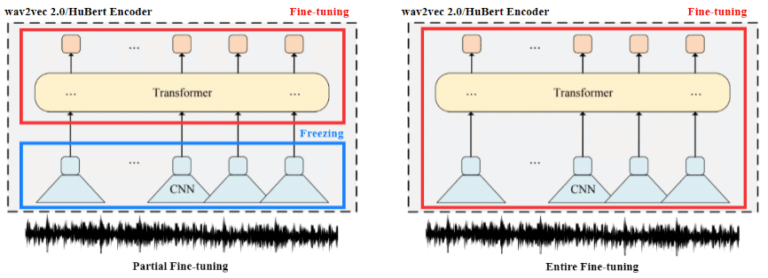
3. Freeze the Feature Encoder: As discussed in the original paper, the CNN feature encoder is already well-trained and robust. Freezing it (setting requires_grad=False for its parameters) prevents it from being updated during fine-tuning. This saves significant GPU memory and can lead to more stable training.

4. Training Arguments: We define all hyperparameters for our training run in a TrainingArguments object. This includes:
   • output_dir: Where to save checkpoints.
   • per_device_train_batch_size: The batch size.
   • learning_rate, num_train_epochs, warmup_steps: Standard training hyperparameters.
   • evaluation_strategy="steps": Evaluate performance every eval_steps.
   • group_by_length=True: A key optimization that groups samples of similar length into batches, minimizing the amount of padding needed and speeding up training significantly.

The video below offers practical advice on setting these arguments, especially managing checkpoints when using cloud environments like Google Colab.

2.4. Training and Evaluation

Finally, we instantiate the Trainer with all the components we've prepared (model, data collator, training arguments, datasets, etc.) and start training with a single command: trainer.train().

During training, you'll see logs that track the training loss and the validation WER. Your goal is to see the WER consistently decrease.

Once training is complete, you can use the best checkpoint to evaluate the final performance on the test set and see how well your model transcribes unseen audio.

---

3. The Power of Pre-training: Fine-Tuning vs. From Scratch

Now we address the second part of our learning outcome: comparing the performance. Just how much benefit does this complex self-supervised pre-training provide? The original wav2vec 2.0 paper gives us the definitive answer.

First, let's read the paper's description of the fine-tuning process, which formalizes what we just implemented.

Low-Resource Scenario

The most stunning results are in low-data settings. Look at Table 1 from the paper, which shows the WER on Librispeech when fine-tuning on very small amounts of labeled data.

From Table 1, the LARGE model pre-trained on the LibriVox dataset (LV-60k) and then fine-tuned on just 10 minutes of labeled data achieves a WER of 4.8% / 8.2% on the Librispeech test sets. This is an incredible result.

Comparison: A model trained "from scratch" (with random weights) on only 10 minutes of data would completely fail to converge. It would have no chance of learning the complex patterns of speech. The WER would likely be near 100%. The ability to achieve a single-digit WER with so little data is entirely due to the knowledge transferred from the 53,000 hours of unlabeled pre-training data.

High-Resource Scenario

What if we have plenty of labeled data? Does pre-training still help? Table 2 in the paper compares models fine-tuned on the full 960 hours of labeled Librispeech data. Crucially, it includes a baseline named "LARGE - from scratch".

The results from Table 2 are clear:

• LARGE - from scratch: Trained on 960 hours of labeled data, it achieves a WER of 2.1% / 4.6%.
• LARGE pre-trained on LV-60k: Pre-trained on 53k hours unlabeled, then fine-tuned on 960 hours labeled, it achieves a WER of 1.8% / 3.3%.

Analysis: Even with nearly 1000 hours of transcribed speech, pre-training still provides a significant performance boost. The knowledge gained from the massive, unlabeled LibriVox dataset allows the model to achieve a lower error rate than a model trained on the labeled data alone.

---

Conclusion

In this lesson, you've walked through the entire pipeline for fine-tuning a state-of-the-art, self-supervised speech model for ASR. We've translated the theory from previous lessons into a practical, repeatable workflow using powerful tools like Hugging Face transformers and datasets.

Key Takeaways:

• Fine-Tuning Workflow: The process involves preparing a labeled dataset, creating a Wav2Vec2Processor (tokenizer + feature extractor), dynamically padding batches with a DataCollator, and configuring a Trainer to handle the training loop.
• Key Configurations: Freezing the CNN feature encoder and using group_by_length are important optimizations for stable and efficient training.
• The Power of Pre-training: The comparison is not even close. Fine-tuning a pre-trained model enables ASR with incredibly small amounts of labeled data (minutes, not thousands of hours), a task that is impossible for models trained from scratch.
• Benefit in All Scenarios: Even when large labeled datasets are available, pre-training on even larger unlabeled corpora still provides a clear performance advantage, leading to lower Word Error Rates.

Preview of the Next Lesson:

We've now seen the power of transfer learning for an ASR task within a single language. But how well do these representations generalize? In the next lesson, we will explore this further by answering the question: How do self-supervised speech models enable transfer learning across different languages and downstream tasks? We'll look at multilingual models like XLSR and see how these representations can be used for tasks beyond ASR.