Cleaning and Validating Market Time-Series Data

Hello again. In the previous lesson, you created a reproducible Python project: a pinned environment, a lockfile, and a Git history that can explain which code produced a result. Now we make that repository useful for real financial data.

Before calculating returns, fitting GARCH models, or testing a trading signal, treat market data as evidence that must be audited. A downloaded CSV can contain absent observations, repeated records, provider-specific missing-value codes, stock-split discontinuities, and values that look wrong but are actually meaningful. Your goal is not to force every dataset into a rectangular table. It is to distinguish valid observations from invalid ones, preserve an audit trail, and apply a defensible resolution policy.

By the end of this lesson, you should be able to build a basic market-data audit that identifies and resolves—or deliberately quarantines—missing values, duplicate timestamps, corporate-action artifacts, and anomalous observations.

---

Begin with a data contract, not a cleaning command

“Cleaning” is an imprecise word. A professional workflow should instead state a data contract: the properties that a valid observation must satisfy for a specific use case.

For daily equity OHLCV data, a minimal contract might be:

Property	Expected rule	Why it matters
Identity	One row per symbol and trading-session timestamp	Prevents double-counting and ambiguous returns
Time	Valid, consistently interpreted timestamps; ordered within each symbol	Ensures observations have a meaningful sequence
Price fields	Open, high, low, and close are positive when present	Negative or zero prices usually require investigation
OHLC relationship	$low\le open\le high$ and $low\le close\le high$	Catches impossible bars
Volume	Nonnegative and in documented units	Prevents invalid liquidity measures
Corporate actions	Split, dividend, and other action metadata are recorded when available	Separates economic events from data errors
Provenance	Vendor, retrieval time, ticker mapping, and adjustment convention are recorded	Makes the dataset interpretable later

The phrase “when present” is important. A missing daily bar can have several meanings:

• the exchange was closed;
• the instrument had not yet listed or had already delisted;
• the vendor failed to supply data;
• the security did not trade during an intraday interval;
• the observation is unavailable because of a provider-specific code.

These cases should not receive the same treatment. A holiday is not a missing observation. A vendor outage is not a zero return. A delisted stock must not disappear silently from a historical universe.

For a NIFTY 50 project, the natural unique key is usually:

$$(\text{symbol},\text{session date})$$

For intraday data, use a timestamp with timezone information and potentially an exchange or venue identifier. Do not assume that “one timestamp” means “one observation” until you define the instrument and market context.

---

Recognize missingness before deciding what to do

In pandas, missing values can appear as NaN, NaT, pd.NA, or None, depending on the column’s type. Importantly, comparing a value directly with a missing-value sentinel is unreliable; use isna() or notna().

A first-pass missingness report should quantify the problem without changing data:

import pandas as pd

df = pd.read_csv("data/raw/nifty_daily.csv")

missing_report = (
    df.isna()
      .sum()
      .rename("missing_count")
      .to_frame()
      .assign(missing_fraction=lambda x: x["missing_count"] / len(df))
      .sort_values("missing_count", ascending=False)
)

print(missing_report)

For a price panel, inspect missingness in two directions:

1. By column: Is one field such as volume or adjusted close systematically incomplete?
2. By symbol and time: Does one asset have a short history, a long terminal gap, or isolated missing days?

A practical summary for a close-price panel is:

coverage = (
    prices.notna()
          .mean()
          .sort_values()
          .rename("observed_fraction")
)

print(coverage.head(10))

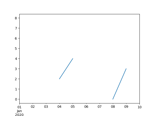
Do not automatically use dropna() after seeing missing values. Dropping every row with any missing value in a multi-asset panel can discard most of the sample. Conversely, filling every missing close can manufacture returns that never occurred.

The plot below shows why this matters. A line chart with breaks is often more honest than a continuous curve produced by interpolation.

A sensible missing-data policy for market prices

For daily close prices used to calculate asset returns:

• Keep missing prices missing in the raw and audited datasets.
• Calculate a return only when both required prices are valid and consecutive according to your intended trading calendar.
• Do not linearly interpolate tradable prices for a backtest or risk model.
• Do not forward-fill a missing close merely to make the table convenient.

Forward-filling a missing price creates artificial zero returns during the gap, followed by one delayed return when trading resumes. Interpolation spreads one price movement across several invented days. Both distort volatility, correlations, drawdowns, and trading signals.

There are legitimate, limited uses of filling:

• A known value such as a static classification code may be forward-filled within a documented validity period.
• A missing observation can be filled for a presentation-only chart if it is visibly marked as imputed.
• A short gap in a non-traded economic series may be handled according to the data’s release schedule.

Those are different tasks from creating a tradable equity return series.

---

Audit timestamps and duplicates before sorting them away

A duplicated date is not always a duplicated observation. It could indicate:

• an accidental repeated file append;
• a vendor revision;
• multiple exchanges or sessions;
• two share classes with an incomplete identifier;
• a corporate-action row mixed with normal trading rows.

First, parse timestamps explicitly. For daily NSE data, preserve the exchange session date carefully; converting a date-only field blindly to UTC can shift its apparent calendar date. For intraday data, store timezone-aware timestamps and document the exchange timezone.

df["timestamp"] = pd.to_datetime(
    df["timestamp"],
    errors="coerce",
)

invalid_timestamps = df["timestamp"].isna()

key = ["symbol", "timestamp"]
duplicate_rows = df[df.duplicated(key, keep=False)].sort_values(key)

print(f"Invalid timestamps: {invalid_timestamps.sum()}")
print(f"Rows in duplicate groups: {len(duplicate_rows)}")

Next, check ordering within each symbol, rather than checking the complete DataFrame:

ordered = df.sort_values(["symbol", "timestamp"]).copy()

is_monotonic = (
    ordered.groupby("symbol")["timestamp"]
           .apply(lambda s: s.is_monotonic_increasing)
)

print(is_monotonic[~is_monotonic])

Resolving duplicates requires evidence

The unsafe shortcut is:

df = df.drop_duplicates(["symbol", "timestamp"], keep="last")

This silently asserts that the last row is correct. Unless the source guarantees row order and you have a trusted revision timestamp, that assertion is unjustified.

Instead, separate duplicate groups into two categories:

1. Exact duplicates: Same key and identical values. Retaining one copy is usually safe, but log the number removed.
2. Conflicting duplicates: Same key but different prices, volume, or action fields. Quarantine them until you can apply a documented source rule.

If your provider supplies a reliable revision_timestamp, a defensible policy can retain the newest revision:

def resolve_revisions(data: pd.DataFrame) -> tuple[pd.DataFrame, pd.DataFrame]:
    key = ["symbol", "timestamp"]
    data = data.copy()

    data["revision_timestamp"] = pd.to_datetime(
        data["revision_timestamp"],
        errors="coerce",
        utc=True,
    )

    duplicate_mask = data.duplicated(key, keep=False)
    duplicate_groups = data.loc[duplicate_mask].copy()

    unresolved = duplicate_groups[
        duplicate_groups["revision_timestamp"].isna()
    ]

    resolvable = data.loc[
        ~duplicate_mask | data["revision_timestamp"].notna()
    ].copy()

    resolved = (
        resolvable.sort_values(key + ["revision_timestamp"])
                  .drop_duplicates(key, keep="last")
    )

    return resolved, unresolved

This function does not pretend every duplicate can be repaired. It returns unresolved rows separately. In a portfolio project, save these records to a review file such as data/interim/quarantined_duplicates.csv, along with your resolution rule in the README.

---

Corporate actions: discontinuity does not necessarily mean loss

A corporate action changes the relationship between a quoted share price and an investor’s economic position. It may therefore create a sharp movement in a raw price series that is perfectly valid.

Consider three examples.

Stock split or bonus issue

Suppose a stock closes at ₹100, then undergoes a 2-for-1 split. Its next quoted price may be ₹50, while each shareholder now owns twice as many shares.

The raw close-to-close price change appears to be:

$$\frac{50}{100}-1=-0.50$$

But the investor has not lost 50% because the number of shares doubled. An adjusted price series rebases historical prices so that this mechanical split does not appear as an economic crash.

A 1:1 bonus issue has the same broad effect: twice as many shares and roughly half the quoted price, all else equal.

Cash dividend

If a share trades at ₹100 and goes ex-dividend with a ₹2 dividend, its price may fall toward ₹98. A price-only return captures that decline. A total-return series should recognize the dividend received by the holder.

Rights issues, buybacks, mergers, and delistings

These events are less amenable to a universal mechanical fix. They can involve eligibility, subscription choices, tender prices, or an actual exit from the dataset. Do not “correct” them solely because their returns are large. Investigate the event and the provider’s stated convention.

Use adjusted prices consistently

Most vendors offer fields such as Close, Adjusted Close, split factors, and dividend amounts. These fields are not interchangeable.

For return research, a common policy is:

• retain vendor-provided raw OHLCV and action data unchanged;
• use a documented adjusted-price field for return calculations when it matches the research objective;
• retain the adjustment convention, vendor, retrieval date, and action fields in metadata;
• never mix raw Open, High, and Low with an adjusted Close in the same price-range calculation unless you have adjusted all fields consistently.

If you download data from an API that includes dividend and stock-split columns, preserve those columns. They provide evidence for explaining a discontinuity later; they are not clutter to discard.

---

Provider conventions can turn “bad values” into valid information

Financial databases often use sentinel codes instead of standard missing values. A negative number may mean “not available,” but it can also have a specific market-data meaning.

For example, CRSP documents special numeric values for unavailable returns and volume. It also documents that a negative PRC can represent an average of bid and ask information rather than an erroneous negative close.

The general rule is:

Decode vendor-specific missing and flag values before applying generic numeric rules.

In a source-specific ingestion step, map known sentinel values to missing values and preserve a flag describing why:

import numpy as np

crsp_return_codes = {
    -44.0: "no_valid_excess_return_comparison",
    -55.0: "no_listing_information",
    -66.0: "no_valid_previous_price",
    -77.0: "off_exchange",
    -88.0: "out_of_range",
    -99.0: "no_valid_price",
}

df["return_status"] = df["RET"].map(crsp_return_codes)
df.loc[df["return_status"].notna(), "RET"] = np.nan

For a different vendor, do not reuse CRSP’s numeric map. Read that vendor’s documentation and create a separate, version-controlled decoding map.

---

Flag anomalies, then investigate them

An invalid value breaks a hard rule. An anomalous value is unusual but potentially real.

Examples of hard failures:

• unparseable timestamp;
• duplicate identity key after applying the source’s documented revision policy;
• negative volume;
• zero or negative price where the data definition forbids it;
• $high<low$;
• a close outside the daily high-low range.

Examples of soft anomaly candidates:

• an unusually large daily return;
• a volume spike;
• a sudden price-scale change;
• a price that sharply diverges from a trusted alternate source;
• a long run of zero volume or unchanged prices.

A large return is not itself a data error. It may reflect an earnings surprise, a takeover announcement, a trading halt, a genuine crash, or a split. Therefore, the right workflow is:

1. Flag the candidate using a transparent rule.
2. Check corporate-action metadata and trading-status information.
3. Compare with an independent legitimate source if available.
4. Correct only a verified data error.
5. Otherwise retain the observation and record the explanation.

For preliminary screening, calculate changes on sorted, unique, positive raw closes and use a robust measure rather than a global mean and standard deviation. A rolling median absolute deviation is less dominated by a single extreme event.

$$z_t^{\mathrm{robust}}=\frac{r_t-\mathrm{median}(r)}{1.4826\mathrm{median}(|r-\mathrm{median}(r)|)}$$

At this stage, you do not need to choose a universal threshold. A threshold such as $|z_t^{\mathrm{robust}}|>8$ is a review trigger, not an automatic deletion rule. The next lesson will formalize simple and log returns; here, the focus is on preventing corrupted inputs from reaching that calculation.

---

Build an auditable first-pass validator

Add a script called scripts/audit_market_data.py to the repository you created previously. The following function identifies quality issues without overwriting the raw data.

from pathlib import Path

import numpy as np
import pandas as pd


KEY_COLUMNS = ["symbol", "timestamp"]
PRICE_COLUMNS = ["open", "high", "low", "close"]


def audit_ohlcv(raw: pd.DataFrame) -> tuple[pd.DataFrame, pd.DataFrame]:
    data = raw.copy()

    data["timestamp"] = pd.to_datetime(
        data["timestamp"],
        errors="coerce",
    )

    for column in PRICE_COLUMNS + ["volume"]:
        data[column] = pd.to_numeric(data[column], errors="coerce")

    has_full_ohlc = data[PRICE_COLUMNS].notna().all(axis=1)

    invalid_price = data[PRICE_COLUMNS].le(0).any(axis=1)
    invalid_volume = data["volume"].lt(0)

    invalid_range = has_full_ohlc & (
        (data["high"] < data[["open", "close"]].max(axis=1))
        | (data["low"] > data[["open", "close"]].min(axis=1))
        | (data["high"] < data["low"])
    )

    duplicate_key = data.duplicated(KEY_COLUMNS, keep=False)
    invalid_timestamp = data["timestamp"].isna()

    data["quality_status"] = "accepted"
    data.loc[invalid_timestamp, "quality_status"] = "invalid_timestamp"
    data.loc[duplicate_key, "quality_status"] = "duplicate_key"
    data.loc[invalid_price, "quality_status"] = "invalid_price"
    data.loc[invalid_volume, "quality_status"] = "invalid_volume"
    data.loc[invalid_range, "quality_status"] = "invalid_ohlc_range"

    summary = (
        data["quality_status"]
        .value_counts(dropna=False)
        .rename_axis("quality_status")
        .reset_index(name="row_count")
    )

    return data, summary


if __name__ == "__main__":
    raw_path = Path("data/raw/nifty_daily.csv")
    audited_path = Path("data/interim/nifty_daily_audited.csv")
    report_path = Path("data/interim/nifty_daily_audit_summary.csv")

    raw = pd.read_csv(raw_path)
    audited, report = audit_ohlcv(raw)

    audited_path.parent.mkdir(parents=True, exist_ok=True)
    audited.to_csv(audited_path, index=False)
    report.to_csv(report_path, index=False)

    print(report.to_string(index=False))

This is intentionally conservative. It labels a row rather than silently deleting it. In a stronger production implementation, use multiple flag columns rather than one quality_status, because one row can be both duplicated and have an invalid range.

Maintain this layered structure:

data/
├── raw/          # Original download; never edited manually
├── interim/      # Parsed, decoded, audited, quarantined records
└── processed/    # Dataset approved for a defined analysis

Your processed dataset should be created only after you state the resolution policy. For example:

Issue	Example resolution
Exact repeated row	Retain one row; log duplicate count
Conflicting repeated rows	Resolve using a documented revision field or quarantine
Provider missing code	Decode to missing value; preserve the reason in a flag
Isolated missing price	Keep missing; do not fabricate a return
Split-related discontinuity	Use consistent adjusted prices and retain split metadata
Invalid OHLC relation	Quarantine, verify against source, then correct or exclude
Large but verified event return	Retain and document it

Commit the script, the small audit summary, and the policy documentation. Do not commit proprietary raw data that you are not licensed to distribute.

---

Key takeaways

Reliable market-data work begins with explicit rules, not dropna() and fillna().

• Define a valid observation through a data contract: identity, timestamps, field relationships, action metadata, and provenance.
• Detect missingness with isna() and interpret gaps using market and vendor context.
• Never interpolate or forward-fill equity prices merely to create a convenient return series.
• Treat duplicate timestamp groups as evidence to examine; resolve them only with a documented source rule.
• Corporate actions can create large raw-price discontinuities without creating an equivalent economic gain or loss.
• Decode provider-specific sentinel values before applying generic anomaly filters.
• Separate impossible values from unusual but potentially genuine market events.
• Preserve raw data, audit outputs, quarantine records, and the reasoning behind every correction.

In the next lesson, you will use the approved price series to calculate simple and logarithmic returns. The quality decisions made here determine whether those returns represent market behavior—or artifacts of the data pipeline.