Constructing a Comprehensive Workload Model

Good to see you again. In the previous lesson, you converted a business objective into a measurable quality-attribute scenario. In particular, the checkout example defined a critical condition: during a flash sale, eligible order submissions should receive a durable acknowledgement within 2 seconds for at least 99.9% of requests, even when the payment provider is temporarily unavailable.

That scenario names an important load condition—200 order submissions per second—but it is not yet a complete basis for evaluating an architecture. We need to understand how demand changes over time, which operations create that demand, how much data each operation moves and retains, which latency measures apply, and what assumptions could invalidate the design later. This is the role of a workload model.

By the end of this lesson, you should be able to write a compact workload model that an architect, product stakeholder, performance engineer, and operations team could all inspect, challenge, and use.

---

A workload model is not “the expected number of users”

A workload model is a quantified description of the demand a system must handle under stated conditions. It is a model, not a prediction of perfect certainty. Its value comes from making uncertainty visible early enough to test and revise it.

A useful model answers five connected questions:

Dimension	Question it answers	Example
Scope and operation mix	Which user journeys and system operations create demand?	Browse product, update cart, submit order
Traffic shape	How does demand vary over time?	A two-hour sale peak, a five-minute launch spike, quieter overnight traffic
Data volume	How much data is transferred, written, replicated, and retained?	A 6 KB order plus event data, retained for seven years
Latency and correctness targets	What user-visible or business-visible behavior must hold at each load level?	Order acknowledgement p99 at or below 2 seconds; no duplicate orders
Growth and uncertainty	What may change, how fast, and how confident are we?	30% annual growth; campaign traffic may double after a new channel launch

“10,000 users” is therefore not enough. Ten thousand users reading a cached catalogue are materially different from ten thousand users submitting orders, uploading videos, or repeatedly refreshing a dashboard. Even the same user journey produces a different workload when user behavior, request size, network location, or traffic concentration changes.

A model should also state its boundary. Are you describing:

• demand at the public API,
• traffic reaching a specific service,
• database reads and writes,
• messages entering an asynchronous pipeline,
• or all of these, separately?

Mixing these boundaries produces misleading calculations. “200 requests per second” at an edge gateway does not mean every downstream dependency receives 200 requests per second.

---

Start with observable demand and explicit assumptions

For an existing system, production telemetry is the best starting point: request counts by operation, response times, error rates, payload sizes, active users, database I/O, message rates, and storage growth. Historical data reveals patterns that stakeholder memory often misses: weekday cycles, payroll-day spikes, regional differences, feature-release effects, or a slow rise in request size.

For a new system, there is no production history. Use market research, comparable products, pilots, business forecasts, and expert judgement—but label each figure as an assumption and give it a confidence level or range. “We expect 50,000 monthly active users” should lead to further questions:

• What fraction will be active on a typical day?
• How often does an active user perform each business operation?
• Is use distributed across a day or concentrated in a few hours?
• Does a campaign create a temporary peak beyond ordinary growth?
• Which number is a contractual commitment, and which is an early estimate?

The purpose is not to manufacture false precision. A rough estimate that correctly identifies a possible two-order-of-magnitude gap is already architecturally valuable. If a first-pass calculation suggests one database can support the expected write rate for years, sharding may not be justified. If it suggests a single campaign could generate more write traffic than the proposed persistence layer can plausibly sustain, that is a design risk to investigate now.

---

Model traffic as a shape, not an average

Traffic has a rate and a shape.

The rate might be requests per second, orders per minute, bytes per second, messages per second, or concurrent sessions. The shape describes how that rate changes over time. An average rate is useful for annual cost or broad storage planning, but it can conceal the conditions that cause latency collapse and errors.

For example, suppose checkout receives 3 million orders per day. Dividing by 86,400 seconds yields an average of roughly 35 orders per second. That average is nearly irrelevant if 1.4 million orders arrive during a two-hour flash sale. During that sale the average is about 200 orders per second, before considering short bursts at the campaign opening.

The peak multiplier is a convenient first expression of that difference:

$$\text{peak rate}=\text{average rate}\times \text{peak multiplier}$$

A multiplier is not an explanation. It must be attached to a cause and a duration. “Peak is 6 times average for 15 minutes after a promotional push” is a usable assumption. “Plan for 6 times average” without a time window is not.

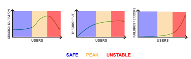
The image illustrates why “maximum throughput” is not automatically a sensible capacity target. Near saturation, a small increase in arrival rate can greatly increase waiting time. Throughput may plateau, while user-visible latency and failure rate worsen. The correct operational limit is usually the highest load at which the system still meets its stated latency and reliability objectives with headroom—not the point just before total failure.

At a minimum, distinguish these traffic shapes:

• Steady state: typical sustained demand, useful for baseline capacity and cost.
• Predictable peak: daily sign-in rushes, scheduled reports, sale events, batch windows, or regional business-hour overlap.
• Burst or spike: a short, sharp increase, such as an app notification, ticket release, or cache expiry event.
• Ramp: a gradual rise, common when a campaign spreads through a population or users join a live event.
• Sustained overload: demand remains beyond intended capacity long enough to exhaust queues, connection pools, or storage throughput.
• Degraded-condition traffic: normal user demand continues while a dependency is slow or unavailable, often creating retries, backlog, or fallback work.

For interactive systems, do not treat concurrent users and request rate as interchangeable. A person might spend 30 seconds reading a product description, generating no server load during that time. Conversely, one automation client might produce hundreds of requests per second. Backend services should generally be modelled in terms of arrival rate by operation, while concurrent users are helpful for representing human sessions and test-client behavior.

---

Express the operation mix

A workload model needs an operation-level view because operations consume resources differently. A catalogue lookup may be cacheable and read-heavy. An order submission may trigger validation, durable writes, a payment call, inventory reservation, an event publication, and an email request. Treating both as a generic “request” hides the architectural forces that matter.

Continue the flash-sale checkout scenario with the following illustrative model. These values are assumptions for teaching purposes, not universal e-commerce benchmarks.

Operation at its measurement boundary	Normal business peak	Flash-sale sustained rate	Opening burst	Main characteristic
Product and price reads at Catalogue API	250 requests/s	1,200 requests/s	1,800 requests/s for 5 min	Read-heavy; data changes relatively infrequently
Cart read or update at Cart API	90 requests/s	500 requests/s	700 requests/s for 5 min	Session-associated state; mix of reads and writes
Order submission at Checkout API	40 requests/s	200 requests/s	300 requests/s for 5 min	Durable, correctness-critical write
Payment authorisation attempt	40 requests/s	200 requests/s	300 requests/s for 5 min	External synchronous dependency in the normal path
Order-created event	40 messages/s	200 messages/s	300 messages/s for 5 min	Durable asynchronous work for downstream consumers

Several observations are immediately possible:

1. The Catalogue API sees six times the checkout rate during the sale. Its dominant concern may be read capacity and cache behavior, not transaction durability.
2. Checkout and payment traffic are correlated in the normal path, but payment may have a different rate during recovery, retries, or partial failure.
3. The event rate should be modelled independently. Downstream consumers might process one order-created event into multiple operations, and their throughput can differ from the producer’s rate.
4. The opening burst is a separate design condition from the two-hour sustained rate. It should not be silently averaged away.

A compact narrative specification for the traffic shape might read:

The weekly flash sale starts at 10:00 local time. Checkout traffic ramps from 40 to 200 order submissions per second during the preceding ten minutes, sustains 200 requests per second for two hours, and reaches 300 requests per second for up to five minutes immediately after opening. The product catalogue receives a higher read rate due to browsing and refresh activity. This model represents authenticated shoppers in the primary region; internal support traffic and bot traffic are excluded.

That final sentence matters. A model becomes reviewable when it says what it excludes. If bot traffic later becomes material, it is an assumption that has failed—not an inexplicable surprise.

---

Quantify data volume in more than one dimension

“An order is 4 KB” is not yet a data-volume model. Architecture decisions depend on several different quantities:

• Ingress and egress bandwidth: bytes sent and received at the public boundary.
• Internal network traffic: service calls, replication, cross-zone traffic, and events.
• Write rate: records, index updates, log entries, and messages created per second.
• Working set: data likely to be held in memory or cache during a time interval.
• Retained storage: data kept for days, years, or indefinitely.
• Recovery and replication load: extra data movement during failover, replay, or rebuilding.

For the checkout model, assume each accepted order produces:

• a 4 KB logical order record;
• a 2 KB durable order-created event;
• 40% additional overhead for indexes and metadata;
• three copies of retained data through replication;
• seven-year order retention.

At the 200 orders-per-second campaign rate, the logical retained-data write rate is:

$$200\text{ orders/s}\times (4+2)\text{ KB/order}=1.2\text{ MB/s}$$

That is not the final storage requirement. It excludes indexes and replicas. The physical retained-data rate under the assumptions is approximately:

$$1.2\text{ MB/s}\times 1.4\times 3=5.04\text{ MB/s}$$

For daily storage planning, use the traffic shape rather than pretending that campaign peak lasts all day. Suppose the system receives 20 orders per second for 22 hours, 200 orders per second for two campaign hours, and the five-minute opening burst adds 30,000 orders above the sustained campaign rate. The daily order count is approximately:

$$(20\times 79,200)+(200\times 7,200)+30,000=3,054,000\text{ orders/day}$$

The physical retained storage per day is then approximately:

$$3,054,000\times 6\text{ KB/order}\times 1.4\times 3\approx 77\text{ GB/day}$$

This estimate is deliberately rough. Its purpose is to expose the high-impact unknowns:

• Are events retained in the same storage tier as orders?
• Does “three copies” include backups, or only live replicas?
• Are attachments, invoices, audit logs, search indexes, and analytics copies included?
• Is data deleted or moved to a cheaper archive tier after a defined period?
• Does the architecture need to support a regional rebuild, and how quickly?

The answer to such questions may change the estimate more than replacing 4 KB with a precisely measured 4.3 KB record ever would.

---

Attach latency targets to the right operation and condition

Latency targets belong in the workload model because latency and load interact. But a latency target needs the same precision as the quality scenarios from the prior lesson.

For each important operation, state:

1. Population: which requests count.
2. Boundary: when timing begins and ends.
3. Statistic: median, percentile, maximum, or another measure.
4. Target: the acceptable value.
5. Condition: the traffic level, region, and dependency condition in which it applies.

For the checkout example:

Operation	Timing boundary	Target during sustained flash-sale load
Catalogue read	Public API receipt to complete API response	p95 at or below 300 ms
Cart update	Public API receipt to durable cart acknowledgement	p95 at or below 500 ms
Eligible order submission	Public API receipt to durable order acknowledgement	p99 at or below 2 s; at least 99.9% successful
Payment-pending reconciliation	Payment provider recovery to order resolution	Every pending order resolved or explicitly flagged within 15 min

Averages are insufficient for user-facing architecture decisions. A 200 ms average can coexist with a painful tail in which a meaningful fraction of users wait several seconds. Percentile targets force the design and its tests to account for that tail.

Latency also supplies a first sanity check on concurrency through Little’s Law:

$$L=\lambda W$$

Here, $L$ is the average number of in-flight operations, $\lambda$ is the arrival rate, and $W$ is the average time an operation spends in the system at the same boundary.

If checkout receives 200 order submissions per second and each took the full 2-second target, the system could have roughly:

$$L=200\text{ requests/s}\times 2\text{ s}=400$$

order submissions in flight. This does not size servers by itself. It does indicate that connection pools, worker pools, memory allocations, and downstream concurrency limits must plausibly tolerate that order of magnitude. More importantly, it shows the dangerous feedback loop under overload: longer response times increase in-flight work, which can increase contention and lengthen response times further.

---

Treat growth and failure as separate workload scenarios

A forecast should not consist of one smooth annual-growth number. It should name the business changes that can alter demand and distinguish sustained growth from temporary surges.

For the checkout system, record planning assumptions such as:

Assumption	Why it matters	Validation signal
Order volume grows 30% per year for the next two years	Determines sustained write, storage, and downstream processing growth	Monthly order volume and active-shopper trend
A new marketing channel can double flash-sale traffic	Determines the short-term peak rate and autoscaling headroom	Campaign registration and traffic-source analytics
Mean order record plus event size remains 6 KB	Determines storage, replication, and recovery volume	Sampled production payload and storage growth
Payment-provider recovery target remains 15 minutes	Determines how quickly backlog must be processed	Provider contract and controlled recovery test
Orders remain retained for seven years	Determines storage tiering and archive strategy	Finance and compliance policy review

The payment-provider outage scenario from the previous lesson adds an especially important workload calculation. If eligible checkout requests continue at 200 orders per second during a 15-minute provider outage, then the system accumulates:

$$200\text{ orders/s}\times 900\text{ s}=180,000\text{ pending orders}$$

If those orders must be reconciled within 15 minutes after recovery while new checkout traffic continues, the reconciliation path must process at least 200 additional orders per second above the ongoing live payment rate, before allowing for failed retries or safety margins. This is not a solution choice; it is a demand consequence of the business policy.

That distinction is central. A workload model states what load the system must safely absorb. Later architectural decisions determine whether that implies queues, rate limits, additional provider capacity, delayed processing, customer messaging, or a different product policy.

---

A reusable workload-model template

Use the following structure in architecture work. Keep it short enough to review, but specific enough to drive calculations and tests.

1. Scope and boundaries

• Critical business journey and named operations
• Regions, client types, and tenant segments included
• Measurement boundaries for public requests, service calls, database operations, and messages
• Explicit exclusions

2. Traffic profile

• Typical sustained rate and normal daily or weekly pattern
• Peak sustained rate, duration, and cause
• Burst rate, duration, and cause
• Operation mix, including read/write proportions
• Concurrent-user model only where human pacing matters

3. Data profile

• Request and response size ranges
• Records or objects produced per operation
• Write rate and retained logical volume
• Index, metadata, replication, backup, and archival assumptions
• Retention, deletion, and recovery requirements

4. Service targets

• Latency percentile and observation boundary per critical operation
• Error-rate, correctness, and durability targets
• Separate targets for normal, peak, and degraded conditions

5. Growth, risks, and evidence

• Forecast horizon and growth scenarios
• Assumptions, ranges, owners, and confidence level
• Source of each number: telemetry, contract, business forecast, experiment, or judgement
• Validation plan: production measurement, prototype, load test, or review date

A workload model is a living architectural artifact. Update it after launches, campaigns, performance tests, and material changes in customer behavior. A model that is visibly revised in response to evidence is more valuable than a detailed spreadsheet preserved unchanged after its assumptions have expired.

---

Key takeaways

A workload model turns a quality-attribute scenario’s operating condition into a quantified and reviewable description of demand.

It should describe:

• traffic shape, including baseline, sustained peak, burst, ramp, and degraded conditions;
• operation mix, rather than a single undifferentiated user or request count;
• data volume across bandwidth, writes, retained storage, replicas, and recovery;
• latency targets with a population, boundary, percentile, threshold, and condition;
• growth assumptions with causes, ranges, evidence, and validation signals.

Use back-of-the-envelope calculations to identify implausible designs and the assumptions that deserve testing. They are not substitutes for measurement or performance testing. Most importantly, preserve the distinction between a demand model and an architectural solution: first quantify what must be handled, then compare credible ways to handle it.

Next, you will represent a distributed system’s responsibilities and trust boundaries with context and container diagrams. Those diagrams will give the workload model a structural home: you will be able to show which people, systems, containers, and external dependencies generate or receive each flow.