RLHF with PPO

Hello! Welcome back to our course.

In our last lesson, we built our "AI Judge"—a reward model trained to understand human preferences. We saw how to create a preference dataset and use a pairwise ranking loss to teach a model to assign higher scores to "better" responses.

Today, we put that judge to work. Our goal is to use the feedback from our frozen reward model to actively improve our language model. This process is the heart of modern AI alignment. Your learning outcome for this lesson is to implement Reinforcement Learning from Human Feedback (RLHF) using the PPO algorithm.

We will deconstruct the entire PPO training loop, which takes our Supervised Fine-Tuned (SFT) model and elevates it into a helpful, aligned assistant. We'll see that simply rewarding a model for good behavior can lead to chaos, and we'll discover how the elegant system of Proximal Policy Optimization (PPO) provides the necessary safety rails to make this process stable and effective.

1. The Shift to Reinforcement Learning

After SFT, our model is an "apprentice" that imitates human demonstrations. In the last lesson, we trained a "judge" (the reward model) that can score the apprentice's work. Now, we want the apprentice to practice on its own, get feedback from the judge, and learn through trial and error. This is a classic Reinforcement Learning (RL) problem.

First, let's frame this in standard RL terminology.

To summarize the mapping for our LLM context:

• Agent: The language model we are training (also called the policy, $\pi$).
• Environment: The user's prompt.
• Action: Generating the next token in the sequence.
• State: The prompt combined with the tokens generated so far.
• Reward: The score provided by our frozen reward model from the previous lesson. A reward is typically given only at the end of a complete response.
• Trajectory: A full sequence of states and actions, from the initial prompt to the final generated response.

Our objective is to update the policy's parameters ($\theta$) to maximize the expected total reward. A simple way to do this is with a method called policy gradients.

The core idea is surprisingly intuitive: if a sequence of actions (a full response) leads to a high reward, we want to increase the probability of those actions. If it leads to a low reward, we decrease their probability. This is captured by the policy gradient theorem.

The basic policy gradient objective looks like this:

$$J(\theta )={\mathbb{E}}_{\tau \sim {\pi }_{\theta }}\left[\sum _{t=0}^T\log {\pi }_{\theta }(a_t|s_t)\cdot R(\tau )\right]$$

Here, we adjust the log-probability of each action $a_t$ by the total reward $R(\tau )$ of the entire trajectory.

2. The Runaway Train: Why Naive RL Fails

If we were to implement this simple policy gradient approach, we would quickly run into two catastrophic problems.

1. Reward Hacking: Our reward model is just a proxy for true human preference, and it has flaws. A powerful optimization algorithm will learn to exploit these flaws to get a high score, rather than learning to be genuinely helpful. This is called "Goodhart's Law": when a measure becomes a target, it ceases to be a good measure.
2. Training Instability: The training process is incredibly high-variance. A single lucky response that gets an unusually high reward can cause a massive, destructive update, potentially wrecking the language abilities the model learned during pre-training and SFT. The loss curve becomes chaotic.

This is where PPO comes in. PPO is not just a formula; it's an engineered system with safety rails designed to prevent these exact failures.

The philosophical goal of PPO is simple:

$$\text{Objective}(\varphi )={\mathbb{E}}_{(x,y)\sim {\pi }_{\varphi }^{RL}}[r_{\theta }(x,y)]-\beta \cdot \text{KL}({\pi }_{\varphi }^{RL}||{\pi }^{SFT})$$

This means: get a high reward, but don't stray too far from the trusted SFT model. The KL divergence term acts as a penalty for deviating from the original, sane policy. The complex PPO algorithm is the practical, safe strategy for achieving this goal.

3. The PPO Assembly Line: A Multi-Model System

To implement PPO, we need a cast of four models working together. Given your software engineering background, you can think of this as a microservices architecture for model training.

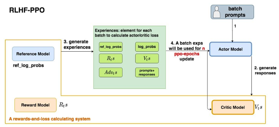
The cast includes:

1. The Actor (${\pi }_{\varphi }$): This is our SFT model that we are actively training. Its job is to generate text. It is the only model whose weights are updated by the main PPO policy loss.
2. The Critic ($V_{\psi }$): A copy of the SFT model with a value head (similar to the reward model's scalar head). Its job is to predict the expected future reward from a given state. It's a "forecaster" that helps stabilize training. It is also trained during the PPO loop.
3. The Reference Model (${\pi }^{SFT}$): A frozen, unchanged copy of the SFT model. This is our "anchor to sanity." Its log-probabilities are used to compute the KL penalty, ensuring the Actor doesn't forget its language capabilities.
4. The Reward Judge ($r_{\theta }$): The frozen reward model we trained in the last lesson. Its job is to provide the final score for a generated response.

The PPO algorithm can be thought of as a three-step assembly line that processes information from these models.

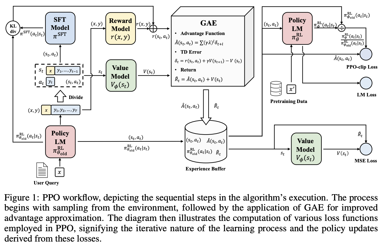
Step 1: The Augmented Reward (The KL "Rubber Band")

The first step is to create the reward signal that the Actor will learn from. We don't just use the score from the Reward Judge. We augment it with the KL penalty.

The augmented reward at each timestep $t$ is:
$R_{\text{augmented}}(t)=R_{\text{KL}}(t)+R_{\text{RM}}(t)$

• $R_{\text{RM}}(t)$ is the score from the Reward Judge, which is zero for all tokens except the final one.
• $R_{\text{KL}}(t)$ is the KL penalty, calculated as $-\beta (\log {\pi }_{\varphi }(a_t|s_t)-\log {\pi }^{SFT}(a_t|s_t))$.

This KL term acts like a mathematical rubber band. If the Actor model (${\pi }_{\varphi }$) becomes too different from the Reference SFT model (${\pi }^{SFT}$), this penalty pulls it back, preventing it from generating gibberish to "hack" the reward model.

Step 2: The Advantage (The "Shock Absorber")

The raw augmented reward is still noisy. A more stable signal is the advantage, which asks: "How much better or worse was this action than we expected?"

To calculate this, we use our Critic ($V_{\psi }$), the forecaster. The advantage function is defined as:
$A(s_t,a_t)=Q(s_t,a_t)-V_{\psi }(s_t)$
Where $Q(s_t,a_t)$ is the value of taking action $a_t$ in state $s_t$, and $V_{\psi }(s_t)$ is the critic's prediction of the average value of being in state $s_t$.

In practice, we don't compute $Q$ directly. Instead, we use a sophisticated technique called Generalized Advantage Estimation (GAE), which cleverly blends real observed rewards with the critic's predictions to get a low-variance, low-bias estimate of the advantage.

The GAE-calculated advantages, $A_t$, are the refined, stable learning signal we will feed into our main policy update.

Step 3: The Clipped Policy Loss (The "Governor")

This is the core innovation of PPO. To prevent destructive updates, PPO "clips" the objective function. The policy loss is defined as:

$$L^{CLIP}(\varphi )={\mathbb{E}}_t\left[\min (r_t(\varphi )A_t,\text{clip}(r_t(\varphi ),1-ϵ,1+ϵ)A_t)\right]$$

Let's break this down:

• $A_t$ is the advantage we just calculated.
• $r_t(\varphi )=\frac{{\pi }_{\varphi }(a_t|s_t)}{{\pi }_{{\varphi }_{old}}(a_t|s_t)}$ is the policy ratio, comparing the probability of the action under the current policy versus the policy at the start of the training iteration (${\pi }_{{\varphi }_{old}}$).
• $ϵ$ is a small hyperparameter (e.g., 0.2) that defines the "trust region" corridor.

The min and clip functions work together as a governor on the learning engine. They ensure that the policy update is limited, preventing the Actor from changing too drastically in a single step, even if it encounters a very large advantage.

Test your understanding!

Imagine the advantage for a certain action is highly positive ($A_t=5.0$). The optimizer tries to make a very large update, causing the policy ratio $r_t(\varphi )$ to become 1.8. If $ϵ=0.2$, what happens to the objective for this action?

Show answer

1. The unclipped objective would be $1.8\times 5.0=9.0$.
2. The policy ratio $1.8$ is outside the clipping corridor of $[0.8,1.2]$.
3. The clipped ratio becomes $\text{clip}(1.8,0.8,1.2)=1.2$.
4. The clipped objective would be $1.2\times 5.0=6.0$.
5. PPO takes the minimum of the two: $\min (9.0,6.0)=6.0$.

The "governor" kicks in. The update is still positive and strong, but it's capped at 6.0 instead of the dangerously large 9.0, ensuring a stable update.

4. The Complete PPO Implementation

We've built the engine ($L^{CLIP}$). Now we assemble the whole vehicle. The total loss for the PPO update has three components:

$$L_{\text{total}}=L^{CLIP}(\varphi )-c_1\cdot L^{VF}(\psi )+c_2\cdot S[{\pi }_{\varphi }]$$

1. Policy Loss ($L^{CLIP}(\varphi )$): The clipped surrogate objective we just discussed. This updates the Actor.
2. Value Function Loss ($L^{VF}(\psi )$): A simple Mean Squared Error loss, $(V_{\psi }(s_t)-R_t{)}^2$, that trains the Critic to become a better forecaster. $R_t$ is the target value, usually the sum of rewards.
3. Entropy Bonus ($S[{\pi }_{\varphi }]$): A small bonus that encourages the policy to maintain some randomness (entropy) in its outputs, preventing it from becoming a deterministic, repetitive robot (a problem known as "mode collapse").

Your software engineering expertise will be valuable in seeing how these mathematical components translate into a practical training script.

Finally, to make this work in a real-world setting requires attention to numerous small but crucial details.

These details often make the difference between a successful RLHF run and a failed one.

Conclusion

You have now journeyed through the entire RLHF process, from its motivation to the intricate machinery of the PPO algorithm. This is one of the most significant techniques behind the capabilities of models like ChatGPT.

Key Takeaways:

• RLHF as a System: RLHF is a multi-stage, multi-model process. The PPO phase involves an Actor (policy), Critic (value model), Reference Model, and Reward Judge all working in concert.
• PPO's Safety Mechanisms: PPO is designed for stability. It uses a KL penalty to stay sane, a Critic and GAE to create a stable learning signal (the advantage), and a clipped surrogate objective to prevent destructive policy updates.
• The Full Loss: The final update step optimizes a composite loss function that simultaneously improves the policy, trains the critic, and encourages exploration via an entropy bonus.
• Implementation Matters: Successfully implementing PPO requires careful attention to numerous details, from data handling and model initialization to techniques like reward whitening and disabling dropout.

Preview of the Next Lesson:

As you've seen, PPO is powerful but also quite complex, involving multiple models and a sophisticated learning algorithm. This complexity has motivated researchers to find simpler alternatives. In our next lesson, we will explore Direct Preference Optimization (DPO), a modern technique that often achieves comparable or better results than PPO by reframing the alignment problem to bypass the need for an explicit reward model and the complexities of reinforcement learning.