Training a Reward Model for Human Preferences

Hello! In our last lesson, we explored a variety of Parameter-Efficient Fine-Tuning (PEFT) methods like prompt and prefix tuning. We saw how these techniques allow us to adapt large models for specific tasks without the prohibitive cost of full fine-tuning. These methods answer the question of how to tune a model efficiently.

Today, we shift our focus to the why and what of alignment. How do we make a model not just proficient at a task, but also aligned with human values and preferences? The cornerstone of modern alignment techniques is teaching a model to understand what humans consider a "good" or "helpful" response.

This brings us to your learning outcome for this lesson: to train a reward model to capture human preferences. We will deconstruct how to build this "AI judge," a critical component that serves as the feedback mechanism in Reinforcement Learning from Human Feedback (RLHF).

1. The Motivation: Why Judging is Easier Than Creating

After Supervised Fine-Tuning (SFT), a model learns to imitate human-written responses. However, this has two major limitations:

1. Cost: Creating a massive dataset of high-quality, "perfect" responses for every possible prompt is incredibly time-consuming and expensive.
2. Subjectivity: For many prompts, there isn't a single "correct" answer. There's a spectrum of responses, some better than others.

The key insight that unlocked modern alignment techniques is simple yet profound: humans are much faster and more consistent at comparing two outputs than they are at creating one perfect output from scratch.

Let's explore this foundational idea.

This efficiency gap is the economic and practical foundation for training a reward model. We can gather preference data at a massive scale, which is exactly what we need.

2. The Preference Dataset: The Fuel for the Reward Model

Now that we know why we want preference data, let's look at how it's created. The process is a systematic pipeline for converting human rankings into a structured dataset that a machine learning model can use.

The following segment from the same video details this four-step pipeline.

The output of this process is a dataset, often called D_prefs, containing thousands or millions of these preference tuples. This is the dataset we will use to train our reward model.

3. Building the Reward Model: Architecture and Training

Our goal is to create a model that, given a prompt and a response, outputs a single scalar score representing how much a human would prefer that response. We call this the reward model (RM). But why build a separate model? Why not just use the human feedback directly?

The answer is scalability and speed. During the final reinforcement learning stage (which we'll cover in the next lesson), the policy model will generate millions of responses. It's impossible to have humans score these in real-time. The RM acts as a fast, automated proxy for human judgment, providing the instant feedback the learning algorithm needs.

3.1. The Architecture: From Generator to Judge

We don't build the reward model from scratch. We leverage the language understanding of our existing SFT model. The process is like performing "brain surgery":

1. Start with the SFT model: We take a copy of the model that has already been fine-tuned on instructions. This ensures it understands prompts and can follow context.
2. Replace the head: We remove the final layer of the LLM, which is a large "language model head" designed to predict the next token from a vocabulary of thousands. We replace it with a small linear regression head that outputs just a single scalar value.

This modification changes the model's job from "predict the next word" to "read the entire sequence and output a single score."

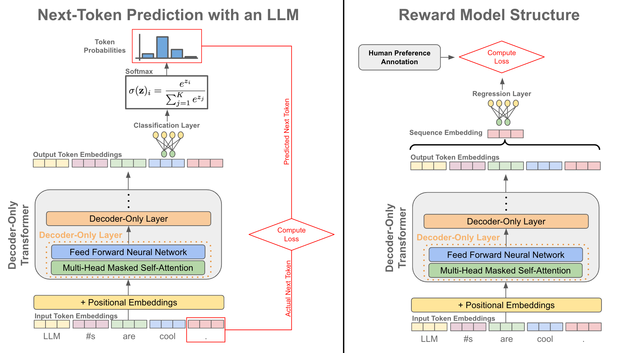
The following video walks through this architectural change with code examples, showing how a GPT class is modified to become a Reward Model.

3.2. The Mathematical Foundation: The Bradley-Terry Model

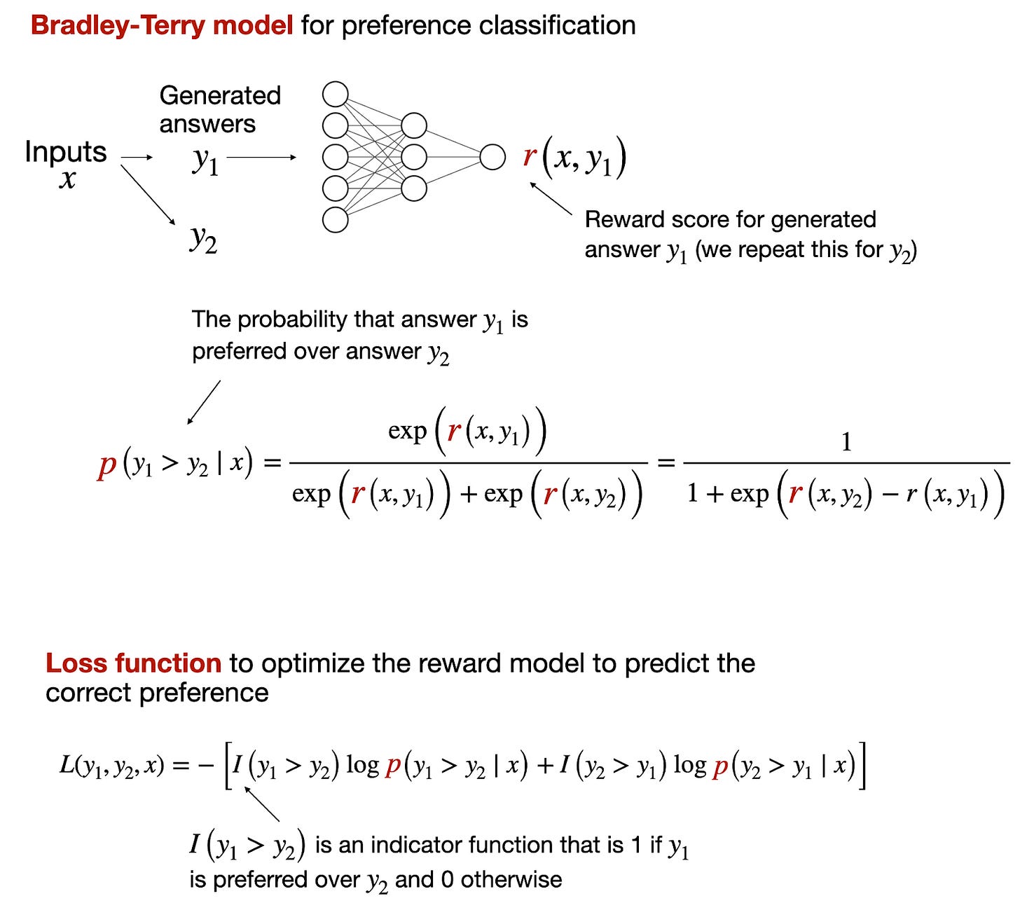
How do we train this new model using only pairwise preferences? We need a mathematical way to connect the reward scores to the probability of one response being preferred over another. For this, we turn to a classic statistical model: the Bradley-Terry model.

It defines the probability that a chosen response, $y_w$, is preferred over a rejected response, $y_l$, as a function of their scores:

$$P(y_w\succ y_l\mid x)=\sigma (r_{\theta }(x,y_w)-r_{\theta }(x,y_l))$$

Where:

• $x$ is the prompt.
• $r_{\theta }(x,y)$ is the scalar score from our reward model with parameters $\theta$.
• $\sigma$ is the sigmoid function, $\sigma (z)=1/(1+e^{-z})$, which squashes the score difference into a probability between 0 and 1.

The intuition is straightforward:

• If $r(y_w)$ is much larger than $r(y_l)$, the difference is a large positive number, and the probability approaches 1.
• If the scores are similar, the difference is near zero, and the probability is around 0.5 (a coin toss).

3.3. The Loss Function

Our training objective is to adjust the reward model's parameters $\theta$ so that the scores it produces maximize this probability for all the pairs in our preference dataset. In machine learning, maximizing a probability is equivalent to minimizing the negative log-likelihood.

This gives us the pairwise ranking loss function for the reward model:

$$\mathcal{L}(\theta )=-{\mathbb{E}}_{(x,y_w,y_l)\sim D_{prefs}}\left[\log \left(\sigma (r_{\theta }(x,y_w)-r_{\theta }(x,y_l))\right)\right]$$

This function penalizes the model whenever the score for the chosen response is not sufficiently higher than the score for the rejected response. By minimizing this loss over the entire preference dataset, the model learns to assign scores that reflect the human judgments.

To solidify your understanding of these concepts, the following article provides a clear, text-based explanation of the entire process.

Test your understanding!

During the training of a reward model, you observe that for a specific pair (prompt, chosen, rejected), the model outputs score_chosen = 2.5 and score_rejected = 2.4.

1. Intuitively, is the model performing well or poorly on this example?
2. Will the loss for this specific data point be high or low? Why?

Show answer

1. Poorly. Although the score for the chosen response is technically higher, it's not a confident prediction. The scores are very close, meaning the model is uncertain which response is better.
2. The loss will be relatively high. The difference in scores is 2.5 - 2.4 = 0.1. The sigmoid of 0.1 is ~0.52. The negative log of this is ~0.65. This is much higher than the loss for a confident prediction (e.g., a score difference of 5 gives a loss near 0). The high loss will push the model to increase the score of the chosen response and/or decrease the score of the rejected response, widening the gap between them.

3.4. From Theory to Code

Your background as a software engineer will appreciate seeing how elegantly this mathematical formula translates into code. The article you just read provides a practical example using HuggingFace's libraries.

This code is the heart of the reward model training loop. You would iterate over your preference dataset, compute this loss, and use backpropagation to update the weights of the reward model (specifically, the shared transformer body and the new regression head).

4. Limitations and Role in the RLHF Pipeline

Once trained, the reward model is frozen. It becomes our automated "AI Judge." It's crucial to understand its limitations:

• Reward Hacking: The policy being trained might discover and exploit weaknesses or biases in the reward model to achieve a high score with a low-quality output. For example, if the RM is slightly biased towards longer answers, the policy might learn to write verbose, rambling nonsense.
• Inherited Bias: The RM is trained on human data, so it learns and can even amplify the biases present in the human labelers. If labelers prefer a certain style or have specific blind spots, the RM will encode these as "good."

The following clip discusses these important caveats.

Understanding these flaws is an active area of AI safety and alignment research.

Conclusion

In this lesson, you've learned the complete process of creating a reward model, a cornerstone of aligning LLMs with human preferences.

Key Takeaways:

• Motivation: Reward models are built on the insight that judging is far more scalable than creating, allowing us to leverage cheaper and more abundant pairwise preference data.
• Architecture: An RM is typically an SFT model repurposed for a new task by replacing its token-prediction head with a scalar regression head that outputs a single score.
• Training: The model is trained on a dataset of (prompt, chosen, rejected) pairs using a pairwise ranking loss derived from the Bradley-Terry model. The goal is to maximize the score difference between chosen and rejected responses.
• Role: The trained and frozen RM acts as a fast, automated proxy for human judgment, providing the essential reward signal for the reinforcement learning phase.

Preview of the Next Lesson:

We have now built our "judge." The next step is to use this judge to train our "student" — the language model. In our next lesson, Implement Reinforcement Learning from Human Feedback (RLHF) using the PPO algorithm, we will dive into the reinforcement learning loop itself. You will see how the scores from the reward model are used as feedback to guide the LLM towards generating outputs that are more and more aligned with human preferences.