One Neural Network Training Step: From Prediction to Parameter Update

Hello. So far, we have separated different kinds of AI product components and distinguished training from validation, deployment, and live inference. The key boundary was that training changes a model’s parameters, while inference normally uses fixed parameters to answer a new request.

Now we open up that training step. By the end of this lesson, you should be able to trace the complete loop: take an input, make a prediction, compare it with the desired answer, determine how each parameter contributed to the error, and adjust those parameters slightly. This is the mechanical core of “learning” in neural networks, including the fine-tuning of many modern models.

---

Training is optimization over parameters

A neural network is a function whose behavior is determined by many adjustable numbers, its parameters:

• weights, which control the strength of connections;
• biases, which shift a unit’s tendency to activate.

Training begins with an example consisting of an input $x$ and a desired target $y$. For a fraud model, the input could be transaction features and the target a later-confirmed fraud label. For a language model, the input is preceding text and the target is the next token that actually followed it.

A single training step has four essential parts:

1. Forward pass: apply the current model to the input to produce a prediction $\hat{y}$.
2. Loss calculation: quantify the gap between $\hat{y}$ and $y$.
3. Backward pass: compute how sensitive the loss is to every parameter.
4. Parameter update: make a small adjustment intended to reduce loss.

The forward pass resembles inference: fixed current weights are applied to an input. The difference is purpose. In inference, the output is returned to a user or downstream system. In training, the output is compared with a known target, and the comparison becomes a signal for modifying the model.

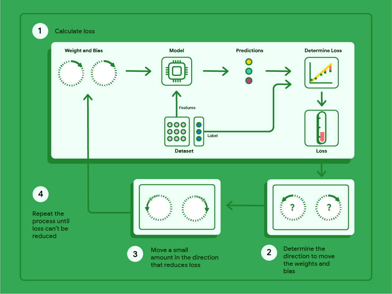
The adjective small matters. Training is not usually a search for a dramatic one-off rewrite of a model. It is a controlled process of many incremental changes, each based on evidence from training examples.

---

A numerical training step: one neuron, one example

To make the full loop visible, start with a deliberately tiny neural network: one linear neuron with one input, one weight, and one bias.

Its prediction rule is:

$$\hat{y}=wx+b$$

Suppose we are training a toy model to predict a normalized numerical outcome. For one training example:

$$x=2,y=2$$

The model currently has:

$$w=0.5,b=0.1$$

1. Forward pass: make the current prediction

Substitute the input and current parameters:

$$\hat{y}=(0.5)(2)+0.1=1.1$$

The model predicts $1.1$, while the desired target is $2$. It is too low by $0.9$.

At this moment, the model has not learned anything. It has merely applied the current parameters, exactly as it would during inference.

2. Loss: convert “wrong” into a usable number

We need a numerical objective that makes a better prediction score lower than a worse prediction. For this example, use squared error with a convenient factor of one-half:

$$L=\frac{1}{2}(\hat{y}-y{)}^2$$

The loss is:

$$L=\frac{1}{2}(1.1-2{)}^2=\frac{1}{2}(-0.9{)}^2=0.405$$

The squaring serves two practical purposes:

• Errors in either direction count positively; being too high and too low are both errors.
• Bigger errors receive disproportionately more penalty.

Terminology varies: teams often call the number for one example the loss, and call the average loss over a batch or dataset the cost or objective. The central idea is unchanged: it is the quantity training tries to reduce.

But the loss alone only tells us how bad the current parameters are. It does not tell us what to change.

---

The gradient: asking which parameter changes matter

For each parameter, we want to know:

If I nudge this parameter slightly upward, does loss rise or fall, and by how much?

The answer is a derivative. For the weight, it is:

$$\frac{\partial L}{\partial w}$$

Read this as: “the sensitivity of loss $L$ to a change in weight $w$.”

In our simple neuron, the prediction depends on the weight through:

$$\hat{y}=wx+b$$

A change in $w$ matters more when the input $x$ is large, because $w$ is multiplied by $x$. The loss depends on the prediction error, which leads to:

$$\frac{\partial L}{\partial w}=(\hat{y}-y)x$$

For the bias:

$$\frac{\partial L}{\partial b}=\hat{y}-y$$

Substitute our example’s values:

$$\frac{\partial L}{\partial w}=(1.1-2)(2)=-1.8$$ $$\frac{\partial L}{\partial b}=1.1-2=-0.9$$

The negative signs are informative. They say that a small increase in either $w$ or $b$ should reduce the loss for this example. That matches intuition: the prediction $1.1$ is below the target $2$, so the model needs to produce a larger output.

The magnitude is informative too. Here, the loss is twice as sensitive to the weight as to the bias:

$$\left|\frac{\partial L}{\partial w}\right|=1.8,\left|\frac{\partial L}{\partial b}\right|=0.9$$

That is because changing the weight affects the prediction through an input of $2$, whereas changing the bias shifts it by only its own amount.

This is the central mental model for a gradient: it is a list of local sensitivity measures, one for every trainable parameter. In a large neural network, that list may contain billions of entries.

---

Gradient descent: turn sensitivities into an update

The general update rule is:

$${\theta }^{\prime }=\theta -\eta \frac{\partial L}{\partial \theta }$$

Here:

• $\theta$ is any parameter, such as a weight or bias;
• $\eta$ is the learning rate, controlling the update size;
• the subtraction means the update moves opposite the direction in which loss increases most quickly.

Let the learning rate be:

$$\eta =0.1$$

We update the weight:

$$w^{\prime }=0.5-(0.1)(-1.8)=0.68$$

Then update the bias:

$$b^{\prime }=0.1-(0.1)(-0.9)=0.19$$

Both have increased, because both gradients were negative.

Now check whether this update improved the model on this same example. Using the updated parameters:

$${\hat{y}}^{\prime }=(0.68)(2)+0.19=1.55$$

The prediction has moved from $1.1$ closer to the target $2$. Its new loss is:

$$L^{\prime }=\frac{1}{2}(1.55-2{)}^2=0.10125$$

The loss declined from $0.405$ to $0.10125$. One update did not make the model perfect, nor was it intended to. It made a locally informed move in a better direction.

Why the learning rate is an important operating choice

A very small learning rate makes training stable but slow. A large one can overshoot the low-loss region, oscillate, or cause training to become unstable.

The same mathematical gradient can therefore lead to very different outcomes depending on the update rule. Modern training systems commonly use more sophisticated optimizers than plain gradient descent, but they retain this essential logic: estimate how parameters affect loss, then alter them in a loss-reducing direction.

---

Backpropagation: efficiently assigning responsibility

The one-neuron example was simple enough to differentiate directly. Real neural networks contain layers of intermediate calculations. A parameter in an early layer influences the final prediction only through all the later layers.

Imagine a simplified chain:

$$x⟶z⟶\hat{y}⟶L$$

For an early weight, training needs to work out how a slight alteration travels through this chain and eventually changes loss. The chain rule gives the structure:

$$\frac{\partial L}{\partial w}=\frac{\partial L}{\partial \hat{y}}\frac{\partial \hat{y}}{\partial z}\frac{\partial z}{\partial w}$$

Each factor captures one local relationship:

• how the loss changes if the prediction changes;
• how the prediction changes if an intermediate value changes;
• how that intermediate value changes if the weight changes.

Backpropagation is the efficient algorithm that applies this logic from the output layer back through the network. It does not literally send error backward through time or alter earlier outputs. Rather, it calculates a useful credit-and-blame signal: how much each weight and bias contributed, locally, to the current loss.

For an output unit that needs to increase, weights from highly active preceding units often deserve larger adjustment, because altering those weights has a larger effect on the output. In hidden layers, several later units may impose competing demands. Backpropagation aggregates those demands and continues working backward.

The useful distinction is:

Term	What it does
Loss function	Defines what “better” means numerically.
Backpropagation	Computes gradients: sensitivity of loss to each parameter.
Gradient descent	Uses those gradients to choose an update direction.
Optimizer	Implements the particular update rule, often extending basic gradient descent.

Founders sometimes use “backpropagation” as shorthand for the whole training process. Technically, it is the gradient-computation component, not the data pipeline, loss design, update rule, or validation process.

---

One example is an explanation, not a production training plan

Our worked update listened to a single example. If a model repeatedly optimized only one example, it would simply memorize that example. The previous lesson’s distinction between training and validation is essential here: a declining training loss is not evidence that the product will handle new cases reliably.

In practice, a training step normally uses a mini-batch, a small collection of examples. The system:

1. performs a forward pass for every example in the mini-batch;
2. computes the average loss;
3. computes gradients of that average loss;
4. updates all parameters once.

Each example has, in effect, a different view about how the parameters should change. Averaging the gradients prevents the model from responding too strongly to any one idiosyncratic case. It does not eliminate noise or guarantee generalization, but it yields an efficient estimate of the direction that should improve performance over the training distribution.

A full pass through the training dataset is called an epoch. Training usually involves many mini-batch updates across many epochs, with validation checks interspersed to detect when lower training loss stops translating into relevant out-of-sample quality.

What changes in a deep network?

The four-part loop is unchanged, even when the scale is enormous:

Tiny example in this lesson	Foundation-model fine-tuning
One numerical input	A sequence of tokenized text, often with additional structured context
One prediction	Probability distributions over possible next tokens
One weight and one bias	Millions or billions of parameters, though some fine-tuning updates only a subset
Squared-error loss	Usually token-level cross-entropy loss
A manually visible derivative	Gradients calculated automatically and in parallel on accelerator hardware

The machinery becomes more elaborate, but “the model learns patterns” ultimately means that repeated parameter updates make its specified training objective lower.

---

An investment lens: what this mechanism does—and does not—establish

Knowing the loop gives you a better way to interpret training claims.

First, training is only as sensible as its target and loss function. A company may have a large dataset, but it needs a credible answer to: what is the desired output for each example? For an AI workflow, useful learning signals might include a verified extraction, an accepted output with minimal edits, a correct routing decision, or a final business outcome. Raw usage logs are not automatically high-quality labels.

Second, lower loss is not automatically greater customer value. Suppose an AI sales assistant achieves lower next-token prediction loss. That does not by itself prove it generates better outbound messages, avoids invented claims, improves reply rates, or reduces human review time. Those require product-specific evaluation measures.

Third, a team should distinguish what is being adjusted:

• Prompt edits, retrieved context, and deterministic rules can substantially improve a product without altering model weights.
• Fine-tuning performs the kind of parameter-update loop described here.
• Pretraining performs it at immense scale, usually beyond the reach or economic rationale of an application startup.

A focused diligence question is:

What trainable parameters are you updating, what target signal defines success, what loss or training objective do you optimize, and how does improvement on that objective show up in a held-out product evaluation?

An early team need not have an elaborate answer to every mathematical detail. But it should be clear whether it is actually training, why the data provides a reliable signal, and why the measured improvement matters to the customer workflow.

---

Key takeaways

A neural-network training step is a repeatable optimization loop:

• The forward pass converts input and current parameters into a prediction.
• A loss function compares that prediction with a target and assigns a numerical penalty.
• Backpropagation calculates how much each weight and bias locally affects that loss.
• Gradient descent or a related optimizer adjusts parameters slightly in the opposite direction to the gradient.
• Practical systems average this signal over mini-batches and validate progress on data not used to fit the model.

The essential claim is modest but powerful: neural-network learning is not a mysterious storage of examples. It is a large number of controlled numerical adjustments that reduce a chosen objective across many examples.

Next, we will move from numerical targets to language. You will interpret an LLM’s next-token output as a probability distribution, and see why sampling produces variation without making a response reliably true.