AC Circuit Analysis: KVL, KCL, and Complex Impedance

Hello! Welcome back to your course on radioelectronics.

In our previous lesson, we established the powerful concept of complex impedance, which unifies the behavior of resistors, inductors, and capacitors under a single framework, $Z$ . We saw how this transforms calculus-based time-domain problems into algebra-based frequency-domain problems.

Introduction

Today's Goal: We will now put that theory into practice. This lesson is dedicated to analyzing complex AC circuits using the same fundamental laws you mastered for DC circuits: Kirchhoff's Current Law (KCL) and Kirchhoff's Voltage Law (KVL). You will learn how to combine impedances in series and parallel and apply systematic methods like mesh analysis to solve for unknown currents and voltages.

By the end of this lesson, you will be able to take a multi-component AC circuit, convert it to its frequency-domain equivalent, and solve it using familiar, powerful techniques, but now with the rigor of complex arithmetic.

Time to complete: Approximately 60 minutes.

1. Combining Impedances: Series and Parallel

Just as resistors can be combined to simplify a DC circuit, impedances can be combined in the same way in an AC circuit. The rules are identical; the only difference is that we are now working with complex numbers.

Series Combination

When components are connected in series, their individual impedances add up to give the total equivalent impedance, $Z_{e q}$ .

Z_{e q} = Z_{1} + Z_{2} + \dots + Z_{n}

For a simple series RLC circuit, the total impedance is:

Z_{e q} = Z_{R} + Z_{L} + Z_{C} = R + jω L + \frac{1}{jω C} = R + j (ω L - \frac{1}{ω C})

Notice how the reactances of the inductor and capacitor directly oppose each other.

Parallel Combination

When components are in parallel, the reciprocal of the equivalent impedance is the sum of the reciprocals of the individual impedances.

\frac{1}{Z _{e q}} = \frac{1}{Z _{1}} + \frac{1}{Z _{2}} + \dots + \frac{1}{Z _{n}}

For the common case of two impedances in parallel, the familiar "product-over-sum" rule applies:

Z_{e q} = \frac{Z _{1} Z _{2}}{Z _{1} + Z _{2}}

A Note on Admittance: To simplify parallel circuit calculations, it's often useful to work with admittance ( $Y$ ), which is the reciprocal of impedance, measured in siemens (S).

Y = \frac{1}{Z} = G + j B

Here, $G$ is the conductance and $B$ is the susceptance. Using admittance, the rule for parallel components becomes a simple sum:

Y_{e q} = Y_{1} + Y_{2} + \dots + Y_{n}

The following video provides a clear, practical strategy for simplifying a circuit by combining series and parallel impedances.

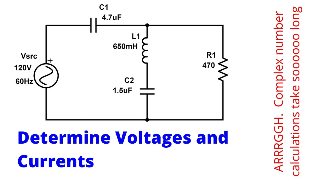
Resource: by ElectronX Lab
Watch: 00:00 - 04:34
Focus on:
- The overall strategy of reducing a complex circuit to a single equivalent impedance.
- The calculations for combining series and parallel impedances. Note how the presenter fluidly moves between rectangular and polar forms to handle addition and multiplication/division of complex numbers.

This process of simplification is the first step in analyzing many circuits. Once you have the total impedance ( $Z_{t o t a l}$ ), you can easily find the total current from the source using the AC version of Ohm's Law: $I_{t o t a l} = V_{so u rce} / Z_{t o t a l}$ .

2. KVL and KCL in the Frequency Domain

Kirchhoff's laws are fundamental principles of conservation (of energy and charge) and they hold true in any linear circuit, including AC circuits analyzed in the frequency domain.

Kirchhoff's Current Law (KCL): The phasor sum of all currents entering and leaving a node must be zero. $k = 1 \sum n I_{k} = 0$
Kirchhoff's Voltage Law (KVL): The phasor sum of all voltage drops and rises around any closed loop must be zero. $k = 1 \sum n V_{k} = 0$

These laws enable us to use powerful, systematic analysis techniques like Nodal Analysis (based on KCL) and Mesh Analysis (based on KVL).

3. Mesh Analysis with KVL: A Worked Example

Mesh analysis is an excellent way to see KVL applied to a multi-loop AC circuit. The procedure is the same as in DC analysis:

Identify the meshes (independent loops).
Assign a mesh current (e.g., $I_{1}, I_{2}, \dots$ ) to each mesh.
Apply KVL around each mesh, writing the voltage drops across impedances using Ohm's Law ( $V = I Z$ ).
Solve the resulting system of linear equations for the unknown mesh currents.

Given your background, you'll appreciate the mathematical rigor of solving the system of equations. The following video provides a fantastic, in-depth example of this entire process, including solving the system using Cramer's rule.

Resource: by RF Design Basics

I recommend watching this video in segments to digest the process:

Setup (00:22 - 05:29): First, focus on how the KVL equations are formulated for each of the three meshes. Observe how shared components contribute terms involving both mesh currents (e.g., $Z (I_{1} - I_{2})$ ). The logic is identical to DC mesh analysis.
Matrix Formulation (05:29 - 07:51): Next, see how the system of three linear equations is organized into a matrix equation of the form $[Z] [I] = [V]$ . This is a standard and powerful representation for circuit equations.
Solving the System (07:51 - 16:33): Finally, watch the process of solving for a specific current ( $I_{2}$ ) using Cramer's rule. This involves calculating the determinants of the main impedance matrix ( $Δ$ ) and a modified matrix ( $Δ_{2}$ ). While in practice you might use a computational tool, understanding the underlying mathematical method is valuable.

This example clearly demonstrates that the core analysis technique remains unchanged—the only new element is the complex arithmetic.

4. The "Work Backwards" Strategy

Once you have solved for primary quantities like total current or mesh currents, you can work your way back through the circuit to find any voltage or current you need. You can use KVL, KCL, and the voltage/current divider rules.

Let's return to the first video, which demonstrates this technique effectively. After finding the total current, the presenter works backward through the equivalent circuits to find the individual voltages and currents.

Resource: by ElectronX Lab
Watch: 04:34 - 06:57
Focus on: How the total current ( $i_{t}$ ) is used to find the voltage across the first-level components. Then, how that voltage is used to find the currents in the next level of parallel branches. This systematic expansion is a crucial skill for practical circuit analysis.

This method, combining impedance simplification with a "work backwards" approach, provides a robust strategy for solving a wide variety of AC circuit problems.

Conclusion

In this lesson, you have connected the theoretical concept of impedance to the practical analysis of AC circuits. You've confirmed that your existing knowledge of KVL, KCL, and systematic methods like mesh analysis are directly applicable in the frequency domain.

Key Takeaways:

Impedances in series add together, while admittances (reciprocals of impedance) add in parallel.
Kirchhoff's laws (KVL and KCL) apply directly to phasor representations of voltages and currents.
Systematic methods like Mesh Analysis (KVL) and Nodal Analysis (KCL) allow you to solve any linear AC circuit by setting up and solving a system of linear equations with complex coefficients.
A powerful analysis strategy involves simplifying a circuit to find a total current/voltage, then working backward to find values for individual components.

What's Next?

Now that we can determine the voltage and current for any component in an AC circuit at a given frequency, we can ask a more interesting question: how does the circuit's behavior change as we vary the frequency? This leads directly to our next topic, "Frequency Response and the Transfer Function," where we will begin to view circuits as filters and systems that shape signals.