Cardiac Output Measurement: Indicator Dilution & Thermodilution

Hello! Welcome back to our course on Medical Instrumentation.

In our last lesson, we explored how to measure blood velocity using electromagnetic and ultrasonic Doppler principles. Today, we move from the speed of blood in a single vessel to the total volume of blood pumped by the entire heart. This is a crucial metric of overall cardiovascular health.

This lesson addresses the learning outcome: Describe indicator dilution and thermodilution methods for measuring cardiac output. We will explore the elegant principle of dilution, where we introduce a known substance or property into the blood and measure how the circulatory system dilutes it to determine flow. This is a cornerstone technique in critical care monitoring.

1. The Principle of Indicator Dilution

Before diving into specific methods, let's understand the core concept that unites them. Cardiac Output (CO) is the volume of blood the heart pumps per minute (in L/min). It's the product of Heart Rate (HR) and Stroke Volume (SV).

The indicator dilution method provides a way to measure CO by applying a principle similar to a classic input-response test. You inject a known quantity of an "indicator" into the bloodstream and measure its concentration downstream as it flows past a sensor.

The fundamental relationship is: The higher the blood flow (Cardiac Output), the more the indicator gets diluted, and the faster it passes the sensor.

To grasp the mathematical basis for this, please read the following sections from the article "Measurement of cardiac output by indicator dilution" on the Deranged Physiology website. It provides a clear, step-by-step explanation.

The Stewart-Hamilton Equation

As you just read, the process culminates in the Stewart-Hamilton equation. In its most basic form, it states:

$\text{Cardiac Output}=\frac{\text{Amount of Indicator Injected}}{{\int }_0^{\infty }c(t)dt}$

Where:

• The numerator is the known quantity of indicator you introduce.
• The denominator, ${\int }_0^{\infty }c(t)dt$, is the area under the concentration-time curve. This represents the total exposure to the indicator as it flows past the sensor.

Think about it intuitively:

• High CO (fast flow): The indicator is swept past the sensor quickly. The concentration curve will be tall and narrow, resulting in a small area. A smaller denominator gives a larger CO.
• Low CO (slow flow): The indicator lingers near the sensor for a longer time. The concentration curve will be short and wide, resulting in a large area. A larger denominator gives a smaller CO.

This inverse relationship between the area under the curve and cardiac output is the key takeaway.

2. Method 1: Dye Dilution

The classic implementation of this principle uses a dye, typically indocyanine green, as the indicator.

To understand how this works in practice, let's watch a short video.

As the video explained, the dye dilution procedure involves:

1. Injection: A known amount of dye is injected rapidly into a central vein (e.g., via a catheter in the vena cava).
2. Mixing: The dye passes through the right heart, lungs, and left heart, mixing with the blood.
3. Sampling: Blood is continuously drawn from a peripheral artery (e.g., the radial artery), and its dye concentration is measured over time by a densitometer.
4. Calculation: A concentration-time curve is plotted. A key challenge is recirculation—the dye starts to appear a second time after circulating through the body. To get the area for just the first pass, the initial downslope of the curve is extrapolated to zero. The cardiac output is then calculated using the Stewart-Hamilton equation.

While historically important, the dye dilution method is now rarely used clinically due to its cumbersome nature and the potential for allergic reactions to the dye. However, it perfectly illustrates the underlying theory.

3. Method 2: Thermodilution

The most common clinical application of the dilution principle is thermodilution. Instead of a dye, the indicator is a change in temperature.

• Indicator: A bolus of cold fluid (usually 10 mL of sterile saline or dextrose solution at room temperature or iced). The "amount" of the indicator is the thermal energy difference between the injectate and the blood.
• Hardware: This method requires a specialized catheter called a Swan-Ganz Pulmonary Artery Catheter (PAC).

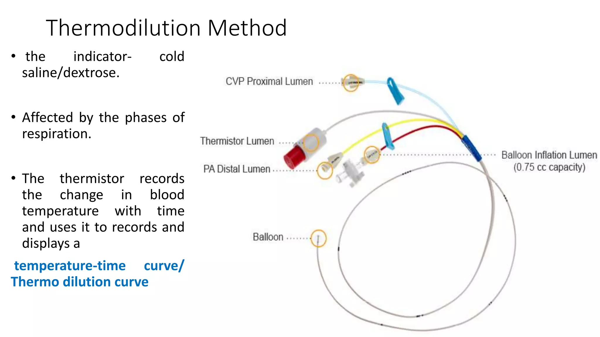
To see how this catheter is placed and how it's used to measure cardiac output, watch the following animation.

The Thermodilution Procedure & Curve

The process, as shown in the video, is:

1. Injection: A known volume of cold saline is injected rapidly into the right atrium via the catheter's proximal port.
2. Mixing & Sensing: The cold bolus travels with the blood through the right ventricle and into the pulmonary artery. A thermistor (a temperature-sensitive resistor) located near the catheter's tip in the pulmonary artery detects the transient drop in blood temperature as the cold bolus flows past.
3. Calculation: A computer connected to the thermistor records the temperature change over time, generating a thermodilution curve. It then calculates the area under this curve and computes the cardiac output using a specific form of the Stewart-Hamilton equation.

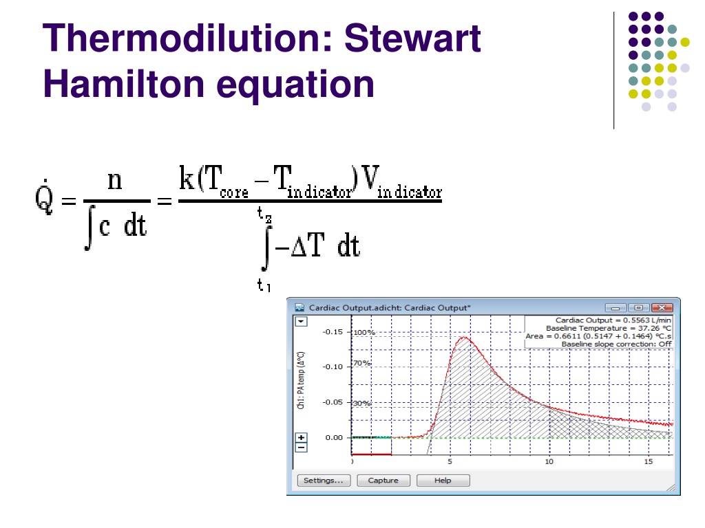
The thermodilution equation, as detailed in the paper "Methods in pharmacology: measurement of cardiac output," is:

$CO=\frac{V_i(T_b-T_i)\cdot K}{\int \Delta T_b(t)dt}$

Where:

• $V_i$ is the volume of injectate.
• $T_b-T_i$ is the temperature difference between the blood and the injectate.
• $\int \Delta T_b(t)dt$ is the area under the thermodilution curve.
• $K$ is a computation constant that accounts for the specific heat and density of the blood and injectate, as well as catheter-specific factors.

This method is the clinical gold standard for measuring cardiac output in critically ill patients because it is safe, repeatable, and less cumbersome than dye dilution. To improve accuracy, typically three separate measurements are taken and averaged.

Conclusion

In this lesson, we explored the principles behind measuring the heart's total flow, or cardiac output, using dilution techniques. These methods are foundational in intensive care and provide a direct window into a patient's hemodynamic status.

Key Takeaways:

• Indicator Dilution Principle: Cardiac output is inversely proportional to the area under the concentration-time curve of an injected indicator.
• Stewart-Hamilton Equation: The formula that mathematically defines this relationship.
• Dye Dilution: The classic method using a dye like indocyanine green, which involves arterial sampling and is complicated by recirculation.
• Thermodilution: The modern clinical standard using a bolus of cold saline as the indicator. It requires a Swan-Ganz pulmonary artery catheter with an injection port and a distal thermistor.
• Thermodilution Curve: The shape of the temperature-time curve provides a visual representation of flow: fast flow gives a narrow, tall curve (small area), while slow flow gives a wide, short curve (large area).

Preview of the Next Lesson:
We have now completed our deep dive into the cardiovascular system, covering pressure, flow velocity, and cardiac output. We will now pivot to a topic that is highly relevant to your work at Neuraease. In the next module, we will begin our study of the Nervous System, starting with the neurophysiological origins of the EEG signal and the standardized methods for acquiring it. This will build the foundation for analyzing brain activity for applications like yours.