Batch Normalization: Stabilizing Neural Network Training

Hello! Welcome to the sixth lesson in our module on Deep Neural Network Fundamentals.

Introduction

In our last lesson, we tackled training instability by learning to diagnose and mitigate exploding gradients. We saw how gradient clipping acts as a crucial reactive safeguard, preventing extreme updates from derailing the learning process. While effective, it's like an emergency brake—it stops a catastrophe but doesn't fundamentally improve the ride quality.

Today, we introduce a technique that is more like a sophisticated suspension system for your neural network: Batch Normalization (BN). Our learning outcome is to implement batch normalization and explain its effect on training stability.

We will explore:

1. The core intuition behind normalizing the inputs to hidden layers.
2. The step-by-step mechanics of the Batch Normalization algorithm.
3. How Batch Normalization transforms training, leading to faster convergence and greater stability.
4. How to implement Batch Normalization in a deep learning framework.

This lesson directly builds on our theme of training stability. While weight initialization gives us a good starting point and gradient clipping saves us from explosions, Batch Normalization continuously re-centers and re-scales the data flowing through the network, making the entire training process smoother and more robust.

1. The Core Idea: Normalizing Hidden Activations

From our first module, you'll recall that normalizing input features is a standard preprocessing step. By scaling inputs to have a mean of zero and a standard deviation of one, we create a more well-behaved optimization problem, often leading to faster convergence.

The key insight behind Batch Normalization, proposed by Sergey Ioffe and Christian Szegedy in 2015, is to ask: If normalizing the network's inputs is so beneficial, why not normalize the inputs to every hidden layer as well?

To understand the motivation, let's watch the first part of a classic lecture by Andrew Ng on this topic.

The problem Batch Normalization aims to solve is what the original authors called Internal Covariate Shift. This refers to the phenomenon where the distribution of each layer's inputs changes during training as the parameters of the preceding layers are updated. This forces each layer to continuously adapt to a "moving target," slowing down the learning process.

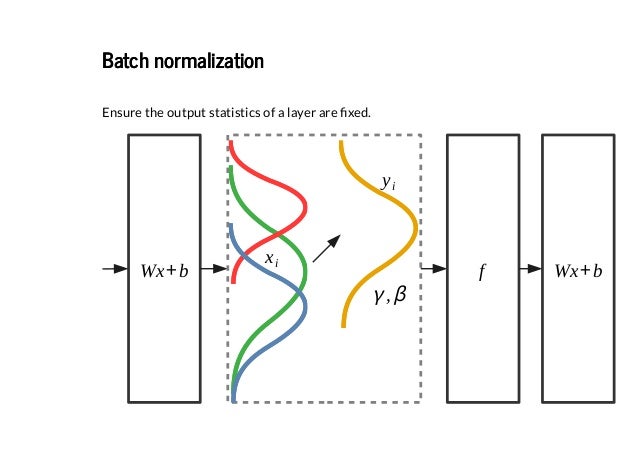
While Internal Covariate Shift was the initial motivation, subsequent research has shown that the primary benefit of Batch Normalization is that it smooths the optimization landscape. This makes the loss function easier for gradient descent to navigate, which in turn allows for higher learning rates and faster convergence.

2. The Mechanics of Batch Normalization

So, how does Batch Normalization actually work? It's a simple, four-step process applied to the pre-activations (often denoted as $z$) of a layer for each mini-batch of data.

Let's continue with Andrew Ng's video, which walks through the algorithm's implementation details.

Here is a summary of the algorithm during training:

For a mini-batch $B=\{z^{(1)},z^{(2)},...,z^{(m)}\}$ of pre-activations for a specific neuron (or feature map channel):

1. Calculate Mini-Batch Mean:
   ${\mu }_B=\frac{1}{m}{\sum }_{i=1}^m{z}^{(i)}$

2. Calculate Mini-Batch Variance:
   ${\sigma }_B^2=\frac{1}{m}{\sum }_{i=1}^m(z^{(i)}-{\mu }_B{)}^2$

3. Normalize: Normalize each pre-activation to have a mean of 0 and a variance of 1.
   ${\hat{z}}^{(i)}=\frac{z^{(i)}-{\mu }_B}{\sqrt{{\sigma }_B^2+ϵ}}$
   The small constant $ϵ$ (e.g., 1e-5) is added for numerical stability to prevent division by zero if the variance is very close to zero.

4. Scale and Shift: The crucial final step. We introduce two new learnable parameters per neuron, $\gamma$ (gamma) and $\beta$ (beta). These are updated via backpropagation just like the network's weights and biases.
   $y^{(i)}=\gamma {\hat{z}}^{(i)}+\beta$
   The value $y^{(i)}$ is the final output of the batch normalization operation, which is then fed into the activation function.

Why are $\gamma$ and $\beta$ necessary?
Forcing all layer inputs to have a mean of 0 and variance of 1 might be too restrictive. For example, for a sigmoid activation function, this would confine most of the inputs to the function's linear region, limiting the network's expressive power. By making the scale ($\gamma$) and shift ($\beta$) learnable, we give the network the flexibility to decide the optimal distribution for each layer's inputs. In the extreme case, if the network learns that $\gamma =\sqrt{{\sigma }_B^2+ϵ}$ and $\beta ={\mu }_B$, it can effectively undo the normalization and recover the original pre-activation $z^{(i)}$.

Test your understanding!

Imagine a mini-batch with 4 pre-activation values for a single neuron: $z=[1,3,5,7]$. Let's assume the learned parameters for this neuron are $\gamma =2.0$ and $\beta =0.5$. (We'll ignore $ϵ$).

1. Calculate the mini-batch mean ${\mu }_B$ and variance ${\sigma }_B^2$.
2. Normalize the third value in the batch, $z^{(3)}=5$.
3. Apply the scale and shift to get the final output $y^{(3)}$.

Show answer

1. Mean: ${\mu }_B=\frac{1+3+5+7}{4}=\frac{16}{4}=4.0$
   Variance: ${\sigma }_B^2=\frac{(1-4{)}^2+(3-4{)}^2+(5-4{)}^2+(7-4{)}^2}{4}=\frac{9+1+1+9}{4}=\frac{20}{4}=5.0$
   The standard deviation is ${\sigma }_B=\sqrt{5.0}\approx 2.236$.

2. Normalize $z^{(3)}$:
   ${\hat{z}}^{(3)}=\frac{z^{(3)}-{\mu }_B}{{\sigma }_B}=\frac{5-4.0}{2.236}\approx 0.447$

3. Scale and Shift:
   $y^{(3)}=\gamma {\hat{z}}^{(3)}+\beta =(2.0\times 0.447)+0.5=0.894+0.5=1.394$
   This value, 1.394, would then be passed to the activation function (e.g., ReLU).

3. Batch Normalization at Test Time (Inference)

A critical question arises: how does this work during inference? We often process a single example at a time, so there is no "mini-batch" to compute a mean and variance from.

The solution is to estimate the "population" statistics during training and use them at test time. This is typically done by keeping an exponentially weighted moving average of the mini-batch means and variances calculated during training.

At inference time, the normalization step becomes:
${\hat{z}}_{test}=\frac{z_{test}-{\mu }_{population}}{\sqrt{{\sigma }_{population}^2+ϵ}}$
And the scale and shift step uses the final learned $\gamma$ and $\beta$ values:
$y_{test}=\gamma {\hat{z}}_{test}+\beta$
This makes Batch Normalization a deterministic operation during inference, simply applying a learned linear transformation to the data.

4. Why is Batch Normalization So Effective?

Now that we understand the mechanics, let's explore its profound effects on training stability and performance.

To summarize and expand on these points:

• Allows for Higher Learning Rates: This is arguably the most significant benefit. By re-normalizing activations at every layer, BN prevents small changes in early layers from getting amplified into massive shifts in later layers. This creates a smoother loss landscape, which allows the optimizer to take much larger, more confident steps without the risk of overshooting or diverging. A quantitative analysis paper ("A Quantitative Analysis of the Effect of Batch Normalization on ...", Cai et al., 2019) has shown that for some problems, BN allows gradient descent to converge even with arbitrarily large learning rates for the weights.

• Reduces Sensitivity to Weight Initialization: Because BN normalizes the outputs of a layer before they are passed to the next, it makes the network far less dependent on the initial scale of the weights. Whether the initial weights are large or small, BN will stabilize the activations, ensuring a reasonable starting point for learning in subsequent layers.

• Acts as a Regularizer: The mean and variance for normalization are calculated on a per-mini-batch basis. This means that the normalization applied to any given example is influenced by the other examples in its batch. This introduces a slight amount of noise into the training process. This noise acts as a form of regularization, slightly reducing the model's reliance on any single training example and improving its ability to generalize. This effect is subtle, but it means you might need less Dropout (our next topic) or other forms of regularization.

5. Implementation in Practice

Adding Batch Normalization to a model is straightforward in modern frameworks like TensorFlow or PyTorch.

Placement:
The standard and most common practice is to place the Batch Normalization layer after the linear (fully connected) or convolutional layer, and before the non-linear activation function.

The flow looks like this:
Linear/Conv Layer -> Batch Norm Layer -> Activation Function

This is because the goal is to normalize the distribution of the pre-activations, $z$, before they are passed into the non-linearity.

Here is how you would define a model with Batch Normalization using tf.keras:

import tensorflow as tf
from tensorflow import keras

# Define the model architecture
model = keras.Sequential([
    # First Conv Block
    keras.layers.Conv2D(32, (3, 3), input_shape=(28, 28, 1)),
    keras.layers.BatchNormalization(), # <-- BN after Conv
    keras.layers.Activation('relu'),    # <-- Activation after BN
    
    keras.layers.MaxPooling2D((2, 2)),
    keras.layers.Flatten(),
    
    # First Dense Block
    keras.layers.Dense(128),
    keras.layers.BatchNormalization(), # <-- BN after Dense
    keras.layers.Activation('relu'),    # <-- Activation after BN
    
    # Output Layer
    keras.layers.Dense(10, activation='softmax')
])

model.summary()

Notice how the BatchNormalization layer is added right after the main computational layers. The framework handles all the logic we discussed: calculating batch statistics during training, updating the moving averages, and using those averages during inference.

Impact of Batch Size:
Since BN relies on mini-batch statistics, its effectiveness is dependent on the batch size. If the batch size is too small (e.g., 2, 4, 8), the calculated mean and variance will be very noisy and may not be a good estimate of the true distribution, potentially hurting performance. For this reason, a batch size of 32 or greater is generally recommended when using BN. For scenarios where small batches are unavoidable (e.g., due to memory constraints with large models), alternatives like Layer Normalization or Group Normalization are often preferred.

Conclusion

You have now added one of the most impactful techniques in modern deep learning to your toolkit. Batch Normalization is a cornerstone of many state-of-the-art architectures, enabling the stable training of very deep networks.

Key Takeaways:

• Core Idea: Batch Normalization applies the principle of input normalization to the inputs of every hidden layer in a network.
• Mechanism: It normalizes pre-activations within a mini-batch to have zero mean and unit variance, then applies a learnable scale ($\gamma$) and shift ($\beta$).
• Inference vs. Training: It uses mini-batch statistics during training and running averages of these statistics during inference.
• Primary Benefits: It smooths the loss landscape, which allows for much higher learning rates and faster convergence. It also reduces the model's sensitivity to weight initialization.
• Regularization: The noise from mini-batch statistics provides a slight regularizing effect.
• Implementation: BN layers are typically placed between the linear/convolutional operation and the activation function.

Preview of the next lesson:
We noted that Batch Normalization has a mild regularizing effect. In our next lesson, we will dive deep into Dropout, a powerful and explicit regularization technique designed specifically to combat overfitting. We will see how it works by randomly "dropping" neurons during training and explore how it complements the stabilization effects of Batch Normalization.