Solving Circuits with Kirchhoff’s Laws

Welcome back. In the previous lesson, you established the sign conventions that make circuit analysis reliable: voltage polarity is a chosen reference, current arrows are chosen references, and a negative result tells you the physical direction is opposite to the chosen arrow. You also used Ohm’s law and the passive sign convention to calculate power.

Now we add the two conservation laws that allow us to solve interconnected circuits:

• Kirchhoff’s Current Law (KCL) governs what happens at nodes.
• Kirchhoff’s Voltage Law (KVL) governs what happens around closed paths.

These laws are the foundation of node-voltage analysis, mesh analysis, DC bias calculations, and eventually MOS amplifier design. A MOSFET bias network may look more complicated than a resistor circuit, but its operating point is still constrained by KCL and KVL.

---

Two laws, one physical idea: conservation

A node is every point connected by uninterrupted ideal wire. Even if a wire bends around the page or has several component terminals attached, it is one node and has one voltage.

Kirchhoff’s Current Law

KCL states that the algebraic sum of currents at a node is zero:

$$\sum i=0$$

Equivalently:

$$\text{total current entering}=\text{total current leaving}$$

KCL follows from conservation of charge. In ordinary lumped circuits, significant charge cannot continuously pile up at a node. If $3\text{mA}$ enters a node, then $3\text{mA}$ must leave it through one or more other branches.

A practical convention for nodal analysis is:

Define every branch current as leaving the node being analyzed, then set their sum equal to zero.

For a resistor between nodes $V_a$ and $V_b$, if you define current from $a$ to $b$, Ohm’s law becomes

$$i_{a\to b}=\frac{V_a-V_b}{R}$$

This expression is especially useful because it works even when you do not yet know which node is at the higher voltage. If the calculated current is negative, actual current flows from $b$ to $a$.

Kirchhoff’s Voltage Law

KVL states that the algebraic sum of voltage changes around any closed path is zero:

$$\sum v=0$$

It is a statement that if you start at one point in a circuit, travel around a closed loop, and return to the same point, your final voltage must equal your starting voltage.

When writing a KVL equation, pick a loop direction and keep it. As you traverse each element:

Element crossing	Signed voltage change
Voltage source from $-$ to $+$	$+V_S$
Voltage source from $+$ to $-$	$-V_S$
Resistor in the assumed current direction	$-iR$
Resistor opposite to the assumed current direction	$+iR$

The key is not guessing the actual current direction perfectly. Choose directions, write equations consistently, and let the algebra decide.

---

One unknown node: KCL becomes a voltage equation

The node-voltage method uses node voltages as the unknowns. This is generally the most useful method for IC analysis because transistor circuits naturally contain many current branches meeting at a few important nodes.

First choose one node as the reference node, or ground:

$$V_{\text{ground}}=0$$

Every other node voltage is measured relative to that reference. Ground does not mean “zero physical energy” or necessarily earth ground; it is simply the chosen zero of voltage.

Consider a circuit with:

• a $12\text{V}$ node connected to an unknown node $V_x$ through $2\text{k}\Omega$,
• a $3\text{k}\Omega$ resistor from $V_x$ to ground,
• a $6\text{k}\Omega$ resistor from $V_x$ to ground.

Write all resistor currents as leaving $V_x$:

$$\frac{V_x-12}{2\text{k}\Omega }+\frac{V_x}{3\text{k}\Omega }+\frac{V_x}{6\text{k}\Omega }=0$$

Multiplying through by $6\text{k}\Omega$ gives

$$3(V_x-12)+2V_x+V_x=0$$ $$6V_x-36=0$$ $$V_x=6\text{V}$$

Now calculate the branch currents:

$$i_{\text{from 12 V}}=\frac{12-6}{2\text{k}\Omega }=3\text{mA}$$ $$i_{\text{through 3 k}\Omega }=\frac{6}{3\text{k}\Omega }=2\text{mA}$$ $$i_{\text{through 6 k}\Omega }=\frac{6}{6\text{k}\Omega }=1\text{mA}$$

The KCL check is immediate:

$$3\text{mA}=2\text{mA}+1\text{mA}$$

The important pattern is that each resistor current is simply the voltage at one end minus the voltage at the other end, divided by resistance. This same pattern will later become the starting point for MOS small-signal node equations.

---

Two unknown nodes: write one KCL equation per node

Now consider a circuit with two unknown node voltages, $V_A$ and $V_B$:

• a known $10\text{V}$ node connects to $V_A$ through $2\text{k}\Omega$;
• $V_A$ connects to ground through $4\text{k}\Omega$;
• $V_A$ connects to $V_B$ through $2\text{k}\Omega$;
• $V_B$ connects to ground through $2\text{k}\Omega$.

Use the “currents leaving” convention at node $A$:

$$\frac{V_A-10}{2\text{k}\Omega }+\frac{V_A}{4\text{k}\Omega }+\frac{V_A-V_B}{2\text{k}\Omega }=0$$

Multiplying by $4\text{k}\Omega$,

$$5V_A-2V_B=20$$

At node $B$,

$$\frac{V_B-V_A}{2\text{k}\Omega }+\frac{V_B}{2\text{k}\Omega }=0$$

Multiplying by $2\text{k}\Omega$,

$$-V_A+2V_B=0$$

The second equation gives

$$V_A=2V_B$$

Substitute into the first:

$$5(2V_B)-2V_B=20$$ $$8V_B=20$$ $$V_B=2.5\text{V}$$ $$V_A=5\text{V}$$

The resistor joining the two unknown nodes carries

$$i_{A\to B}=\frac{V_A-V_B}{2\text{k}\Omega }=\frac{5-2.5}{2\text{k}\Omega }=1.25\text{mA}$$

Because this result is positive, the assumed direction from $A$ to $B$ was correct.

A node-analysis workflow

For basic resistor circuits, use this procedure:

1. Identify all distinct nodes.
2. Choose a reference node and set it to $0\text{V}$.
3. Label every unknown node voltage.
4. Use any voltage source connected to ground to identify a known node voltage immediately.
5. At each unknown node, write KCL.
6. Express each resistor current as a node-voltage difference divided by resistance.
7. Solve the simultaneous equations.
8. Calculate individual branch currents and verify KCL.

A useful structural check: in an equation for $V_A$, the coefficient multiplying $V_A$ comes from all conductances connected to node $A$. Terms involving neighboring node voltages usually have negative signs when all currents are written as leaving the node.

---

Loop analysis with KCL and KVL

Some circuits are more naturally solved by defining branch currents and writing loop equations. The diagram below shows a circuit with two loops and a central junction $b$.

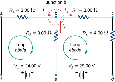
At node $b$, the labelled currents satisfy

$$I_1=I_2+I_3$$

This is KCL: the current arriving from the left equals the algebraic sum of the currents leaving through the downward and right-hand branches.

Now write KVL around the left loop $abefa$, traversed clockwise. The $24\text{V}$ source is crossed from its negative to its positive terminal, so it is a rise. Both resistors are crossed in their assumed current directions, so they are drops:

$$24-3I_1-3I_2=0$$

For the right loop $ebcde$, traversed clockwise:

• crossing $R_2$ upward is opposite to $I_2$, giving $+3I_2$;
• crossing $R_3$ and $R_4$ in the direction of $I_3$ gives drops;
• crossing the $29\text{V}$ source from $+$ to $-$ gives a drop.

Therefore,

$$3I_2-3I_3-4I_3-29=0$$

or

$$3I_2-7I_3=29$$

We now have three equations:

$$I_1=I_2+I_3$$ $$24-3I_1-3I_2=0$$ $$3I_2-7I_3=29$$

Substituting the KCL relation into the left-loop equation gives

$$24-3(I_2+I_3)-3I_2=0$$ $$2I_2+I_3=8$$

Solving with the right-loop equation yields

$$I_2=5\text{A}$$ $$I_3=-2\text{A}$$ $$I_1=3\text{A}$$

The negative result for $I_3$ is meaningful. It says that the actual current in the right branch is $2\text{A}$ opposite to the arrow drawn in the diagram: it flows upward through $R_4$ and leftward through $R_3$.

Nothing has “failed” because the direction assumption was opposite to reality. In fact, retaining the original reference arrow and reporting $I_3=-2\text{A}$ is often the clearest and most rigorous answer.

Both laws check:

$$I_1=I_2+I_3$$ $$3=5+(-2)$$

For the left loop,

$$24-3(3)-3(5)=0$$

For the right loop,

$$3(5)-7(-2)-29=0$$

---

Choosing between node and loop methods

Both methods solve the same physical circuit, and both ultimately use KCL, KVL, and element laws. The choice is about efficiency.

Circuit feature	Usually convenient method
Several current sources or many branches meeting at nodes	Node-voltage analysis
Several voltage sources in simple planar loops	Loop or mesh analysis
Circuit with few unknown node voltages	Node-voltage analysis
Circuit with few independent meshes	Mesh analysis

For integrated circuits, node-voltage analysis becomes particularly important. A common-source amplifier, differential pair, or current mirror often contains several transistor currents meeting at a high-impedance output node. KCL at that node is central to finding gain, output resistance, and transient behavior.

One important distinction:

• A loop is any closed path.
• A mesh is a loop that contains no other loops inside it.

In a planar two-window circuit, the two interior meshes provide independent equations. Writing an equation around the large outside loop usually adds no new information; it can be formed by combining the two interior-loop equations.

---

Debugging and verification

Circuit analysis errors are often bookkeeping errors rather than algebra errors. Use these checks systematically.

Check node equations

At every node, confirm that the signed branch currents sum to zero:

$$\sum i_{\text{leaving}}=0$$

A negative branch current means that current enters the node despite being defined as leaving.

Check loop equations

Around each independent loop, confirm that all voltage rises and drops sum to zero:

$$\sum v=0$$

If your computed currents are correct but a loop does not balance, a source polarity or resistor-drop sign is probably wrong.

Check resistor behavior

For a resistor between nodes $V_a$ and $V_b$,

$$i_{a\to b}=\frac{V_a-V_b}{R}$$

If $V_a>V_b$, the current calculated in the $a$-to-$b$ direction should be positive. Also, a positive physical resistor must dissipate nonnegative power:

$$p_R=i^{2}R\ge 0$$

These checks will remain valuable when the resistors are replaced by MOSFET small-signal resistances and controlled current sources.

---

Key takeaways

KCL expresses charge conservation at a node:

$$\sum i=0$$

KVL expresses voltage consistency around a closed path:

$$\sum v=0$$

For node-voltage analysis, choose a ground node, label unknown node voltages, write each resistor current as a voltage difference divided by resistance, and apply KCL once for each unknown node.

For loop analysis, assign current references, write KCL at junctions as needed, then write KVL around independent loops. A negative current result does not indicate an error; it tells you that the actual current direction is opposite to your chosen reference arrow.

Next, you will use these same laws to derive Thévenin and Norton equivalents, which let you replace a complicated linear network with a simple source-and-resistance model at a selected port.