Darcy-Weisbach & Moody Chart: Major Head Loss

Hello! Welcome to your next lesson in the Fluid Mechanics module.

In our last session, we explored Bernoulli's equation, a powerful tool for analyzing ideal, frictionless fluid flow. We also highlighted its major limitation: real-world flows always involve friction, which causes a loss of energy that the simple Bernoulli equation can't account for. The preview for this lesson mentioned we would tackle this by quantifying frictional losses.

Today, we'll do exactly that. We will focus on major losses—the energy losses that occur due to friction between the fluid and the internal surface of a pipe over its length. This is a critical concept in engineering, as it dictates how much power is needed to pump fluids, whether it's water in a city network, fuel in an aircraft's supply line, or oil in a pipeline.

Your learning outcome for this lesson is to calculate major head loss in pipes due to friction using the Darcy-Weisbach equation and Moody chart.

1. From Ideal to Real Flow: Quantifying Head Loss

In the last lesson, we wrote Bernoulli's equation for ideal flow between two points as:
$\frac{P_1}{\rho g}+\frac{v_1^2}{2g}+z_1=\frac{P_2}{\rho g}+\frac{v_2^2}{2g}+z_2$
Each side represents the total "head" or energy per unit weight at that point. In a real pipe with friction, energy is lost as the fluid moves from point 1 to point 2. We account for this by adding a head loss term, $h_L$, to the equation, which is often called the Extended Bernoulli Equation:
$\frac{P_1}{\rho g}+\frac{v_1^2}{2g}+z_1=\frac{P_2}{\rho g}+\frac{v_2^2}{2g}+z_2+h_L$
The primary tool for calculating this major head loss is the Darcy-Weisbach equation.

As you saw in the reading, the Darcy-Weisbach equation is:
$h_L=f\frac{L}{D}\frac{v^2}{2g}$
Where:

• $h_L$ is the major head loss (in meters or feet).
• $f$ is the Darcy friction factor (dimensionless).
• $L$ is the length of the pipe.
• $D$ is the diameter of the pipe.
• $v$ is the average velocity of the fluid.
• $g$ is the acceleration due to gravity.

In this equation, $L,D,v,$ and $g$ are usually known or can be easily calculated. The entire challenge lies in determining the friction factor, $f$.

2. The Friction Factor, $f$

The friction factor isn't a constant; it depends on the flow conditions. The first step is always to calculate the Reynolds number ($Re$) to determine if the flow is laminar or turbulent.
$Re=\frac{\rho vD}{\mu }=\frac{vD}{\nu }$
Where $\rho$ is density, $\mu$ is dynamic viscosity, and $\nu$ is kinematic viscosity.

Laminar Flow ($Re\lesssim 2300$)

For laminar flow, the situation is simple. The friction factor depends only on the Reynolds number. The derivation is shown in the resource you just read, but as per your preference, we can jump straight to the result.

For laminar flow, the friction factor is given by a direct calculation:
$f=\frac{64}{Re}$
Notice that the pipe's surface roughness does not play a role in laminar flow.

Turbulent Flow ($Re\gtrsim 4000$)

For turbulent flow, things get more complex. The friction factor now depends on both the Reynolds number and the pipe's surface roughness. This is where we need a graphical tool: the Moody chart.

3. The Moody Chart

The Moody chart is a log-log plot that relates the three crucial quantities for turbulent flow:

1. Reynolds Number ($Re$) on the horizontal axis.
2. Relative Roughness ($ϵ/D$) represented by the family of curves.
3. Darcy Friction Factor ($f$) on the vertical axis.

The relative roughness, $ϵ/D$, is the ratio of the mean height of roughness of the pipe ($ϵ$) to the pipe diameter ($D$). The absolute roughness $ϵ$ is a property of the pipe material, which you can find in a table.

Here is a table with typical roughness values for new, clean pipes.

Material	Roughness, $ϵ$ (mm)	Roughness, $ϵ$ (ft)
Glass, Plastic	0 (smooth)	0 (smooth)
Copper or Brass Tubing	0.0015	0.000005
Commercial Steel or Wrought Iron	0.045	0.00015
Stainless Steel	0.002	0.000007
Galvanized Iron	0.15	0.0005
Cast Iron	0.26	0.00085
Concrete	0.9 - 9	0.003 - 0.03

Table adapted from "The Moody Chart" (resource LINK) and other standard fluid mechanics texts.

Now, let's look at the chart itself.

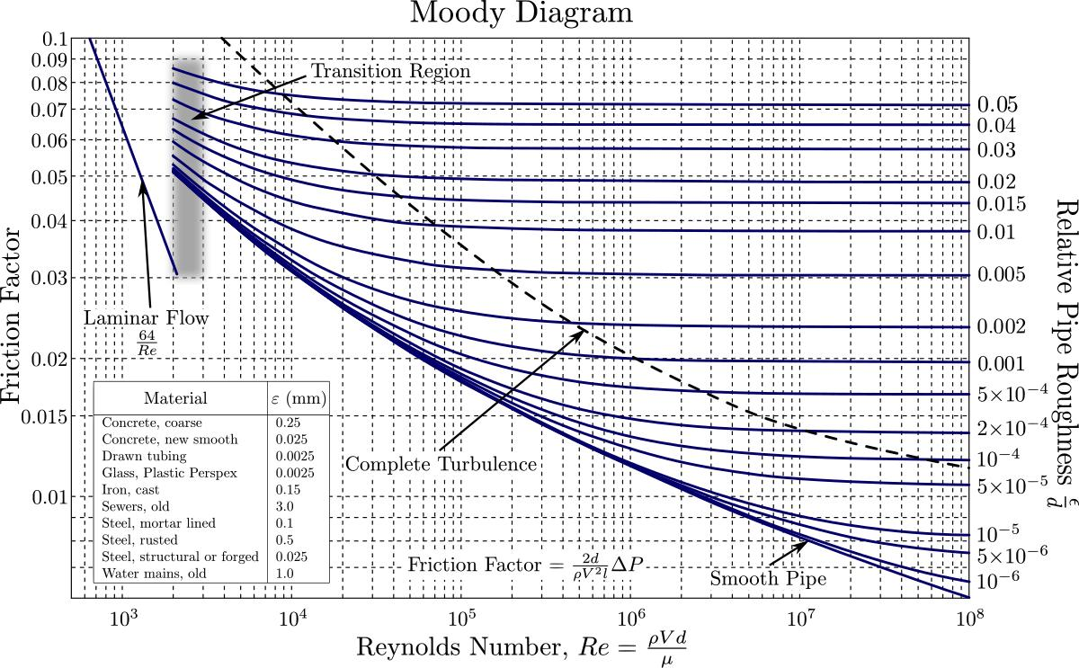
From your electronics background, you can think of using this chart as being analogous to using the characteristic curves of a transistor. For a transistor, you use input parameters like base current ($I_B$) and collector-emitter voltage ($V_{CE}$) to find the resulting collector current ($I_C$) from its curves. Here, you use fluid parameters like Reynolds number ($Re$) and relative roughness ($ϵ/D$) to find the friction factor ($f$) from the Moody chart. It's a graphical method for solving a complex, non-linear relationship.

4. How to Use the Moody Chart: A Worked Example

The best way to learn this is to see it in action. The following video works through a problem with two different velocities, one resulting in laminar flow and the other in turbulent flow. This clearly demonstrates the entire process for both cases.

5. Summary of the Calculation Process

As you saw in the video, the step-by-step process to find the major head loss is as follows:

1. Identify Knowns: Determine the pipe length ($L$), diameter ($D$), material (for roughness $ϵ$), and fluid properties ($\rho ,\mu$ or $\nu$).
2. Calculate Velocity ($v$): If you're given the flow rate $Q$, calculate the velocity using the continuity equation: $v=Q/A$, where $A=\pi D^2/4$.
3. Calculate Reynolds Number ($Re$): Compute $Re=\rho vD/\mu$.
4. Determine Flow Regime:
   • If $Re\lesssim 2300$, the flow is laminar. Proceed to step 5a.
   • If $Re\gtrsim 4000$, the flow is turbulent. Proceed to step 5b.
   • If it's in the transition region ($2300<Re<4000$), the flow is unpredictable. For most engineering problems, it's conservatively treated as turbulent.
5. Find the Friction Factor ($f$):
   • 5a (Laminar): Calculate $f$ directly: $f=64/Re$.
   • 5b (Turbulent):
     i. Find the absolute roughness $ϵ$ from the table for your pipe material.
     ii. Calculate the relative roughness $ϵ/D$.
     iii. On the Moody chart, find your $Re$ on the x-axis.
     iv. Find the curve corresponding to your $ϵ/D$ (you may need to estimate between two curves).
     v. Follow the vertical line from $Re$ up to the $ϵ/D$ curve, then move horizontally to the left to read $f$ from the y-axis.
6. Calculate Head Loss ($h_L$): Substitute the value of $f$ you found, along with $L,D,$ and $v$, into the Darcy-Weisbach equation: $h_L=f\frac{L}{D}\frac{v^2}{2g}$.

Test your understanding!

Water at 20°C ($\rho =998{\text{ kg/m}}^3,\nu =1.004\times 10^{-6}{\text{ m}}^2/\text{s}$) flows at a rate of $Q=0.05{\text{ m}}^3/\text{s}$ through a 300-meter long commercial steel pipe with an internal diameter of 15 cm.

Calculate the major head loss, $h_L$. Use the Moody Diagram provided in the lesson.

Show answer

1. Identify Knowns:

   • $L=300\text{ m}$
   • $D=0.15\text{ m}$
   • Pipe material: Commercial steel
   • Fluid properties: $\rho =998{\text{ kg/m}}^3,\nu =1.004\times 10^{-6}{\text{ m}}^2/\text{s}$

2. Calculate Velocity ($v$):

   • Area $A=\frac{\pi D^2}{4}=\frac{\pi (0.15{)}^2}{4}\approx 0.0177{\text{ m}}^2$
   • $v=\frac{Q}{A}=\frac{0.05{\text{ m}}^3/\text{s}}{0.0177{\text{ m}}^2}\approx 2.82\text{ m/s}$

3. Calculate Reynolds Number ($Re$):

   • $Re=\frac{vD}{\nu }=\frac{(2.82\text{ m/s})(0.15\text{ m})}{1.004\times 10^{-6}{\text{ m}}^2/\text{s}}\approx 421,315$
   • We can write this as $4.21\times 10^5$.

4. Determine Flow Regime:

   • Since $Re>4000$, the flow is turbulent.

5. Find Friction Factor ($f$) using the Moody Chart:

   • Absolute Roughness ($ϵ$): From the table, for commercial steel, $ϵ=0.045\text{ mm}=0.000045\text{ m}$.
   • Relative Roughness ($ϵ/D$): $\frac{ϵ}{D}=\frac{0.000045\text{ m}}{0.15\text{ m}}=0.0003$.
   • Use the Chart:
     i. Find $Re\approx 4.2\times 10^5$ on the x-axis.
     ii. Find the curve for $ϵ/D=0.0003$. This curve isn't explicitly drawn, so we'll need to estimate its position between the curves for 0.0002 and 0.0004.
     iii. Following the vertical line from $Re\approx 4.2\times 10^5$ up to our estimated curve, and then moving left to the y-axis, we read a value for $f$ of approximately 0.016.

6. Calculate Head Loss ($h_L$):

   • $h_L=f\frac{L}{D}\frac{v^2}{2g}=(0.016)\frac{300\text{ m}}{0.15\text{ m}}\frac{(2.82\text{ m/s}{)}^2}{2(9.81{\text{ m/s}}^2)}$
   • $h_L=(0.016)\times (2000)\times \frac{7.9524}{19.62}$
   • $h_L=32\times 0.405\approx 12.96\text{ m}$

The major head loss over the 300 m length of pipe is approximately 13 meters. This means the fluid loses an amount of energy equivalent to being dropped from a height of 13 meters.

Conclusion

In this lesson, we bridged the gap between ideal and real fluid flow by learning how to calculate the energy lost to friction in pipes.

Key Takeaways:

• Friction in pipes causes a major head loss ($h_L$), which is accounted for in the Extended Bernoulli Equation.
• The Darcy-Weisbach equation ($h_L=f\frac{L}{D}\frac{v^2}{2g}$) is the primary tool for calculating this loss.
• The Darcy friction factor ($f$) is the key parameter to determine.
• For laminar flow ($Re\lesssim 2300$), the friction factor is found with a simple formula: $f=64/Re$.
• For turbulent flow ($Re\gtrsim 4000$), the friction factor depends on both the Reynolds number ($Re$) and the relative pipe roughness ($ϵ/D$), and is found graphically using the Moody chart.

Next Steps:
The head loss we calculated today is called "major loss" because, in long pipe systems, it's the dominant form of energy loss. However, real systems also have bends, valves, expansions, and contractions. These components cause additional, localized losses known as minor losses. In our next lesson, we will learn how to calculate these minor losses, allowing us to analyze the total head loss in a complete, realistic piping system.