Common Probability Distributions and Their Applications

Hello! Welcome to your next lesson on the mathematical foundations of AI.

In our last session, we explored Bayes' theorem and saw how it provides a formal framework for updating our beliefs in light of new evidence. We ended with a key question: how do we mathematically represent these beliefs and likelihoods, like $P(\text{Hypothesis})$ or $P(\text{Evidence}|\text{Hypothesis})$? The answer lies in probability distributions.

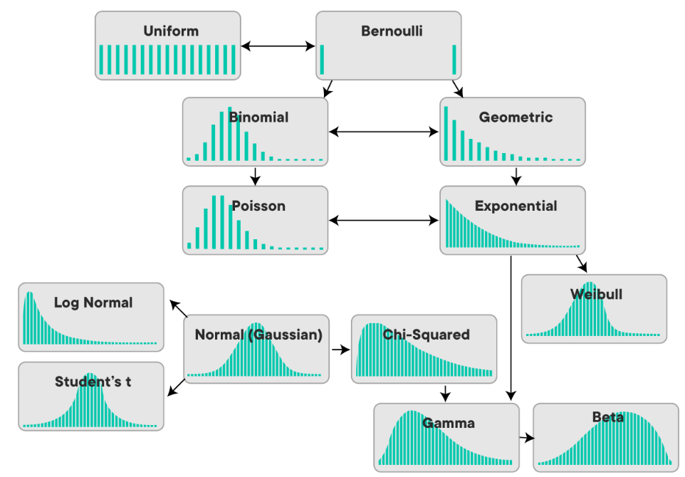
This lesson will address the learning outcome: Describe common probability distributions (Gaussian, Bernoulli, Categorical) and their applications. These three distributions are fundamental building blocks in machine learning. You'll find them everywhere, from defining the outputs of classifiers to modeling noise in your data. Understanding them is crucial for building and interpreting AI models.

1. What is a Probability Distribution?

At its core, a probability distribution is a mathematical function that describes the likelihoods of different possible outcomes for a random variable.

For a deeper look into the formal definitions, please read the first two sections of the following article.

To summarize the key ideas:

• Random Variable (X): A variable whose value is a numerical outcome of a random phenomenon.
• Discrete Random Variable: Can only take on a countable number of distinct values (e.g., the result of a dice roll, the number of clicks on an ad).
• Continuous Random Variable: Can take on any value within a given range (e.g., a person's height, the temperature of a room).
• Probability Mass Function (PMF): For a discrete variable, the PMF, $P(X=x)$, gives the probability that the variable takes on a specific value $x$. The sum of probabilities over all possible values is 1.
• Probability Density Function (PDF): For a continuous variable, the PDF, $f(x)$, describes the relative likelihood of the variable taking on a value near $x$. The probability of the variable falling within a specific range is the integral (area under the curve) of the PDF over that range. The total area under the curve is 1.

Now, let's explore the three key distributions for this lesson.

2. Discrete Distributions: Modeling Choices

Discrete distributions are used to model outcomes that fall into distinct categories.

The Bernoulli Distribution: A Single Yes/No Decision

The Bernoulli distribution is the simplest of all. It models a single experiment with only two possible outcomes, typically labeled as "success" (1) and "failure" (0).

To build your intuition, let's watch a short video segment.

As the video explained, the Bernoulli distribution is defined by a single parameter, $p$, which is the probability of success. Its PMF can be written elegantly as:
$P(k|p)=p^k(1-p{)}^{1-k}\text{for }k\in \{0,1\}$
If $k=1$ (success), the formula becomes $p^1(1-p{)}^0=p$. If $k=0$ (failure), it becomes $p^0(1-p{)}^1=1-p$.

Application in Machine Learning: Binary Classification
The Bernoulli distribution is the probabilistic foundation for binary classification. When a model like logistic regression outputs a probability (e.g., "0.8 chance of being spam"), it's providing the parameter $p$ for a Bernoulli trial. The actual outcome (spam or not spam) is the result of that trial.

This connection is crucial for understanding why certain loss functions are used.

This is a powerful insight: training a binary classifier by minimizing cross-entropy is equivalent to finding the model parameters that make the observed labels most likely, assuming the outcomes are generated from a Bernoulli distribution.

The Categorical Distribution: A Single Choice Among Many

What if an experiment has more than two outcomes, like rolling a die? This is where the Categorical distribution comes in. It generalizes the Bernoulli distribution for a single trial with $K$ possible outcomes.

The Categorical distribution is parameterized by a vector $\vec{p}=(p_1,p_2,\dots ,p_K)$, where $p_i$ is the probability of the $i$-th outcome, and ${\sum }_{i=1}^K{p}_i=1$.

Application in Machine Learning: Multi-class Classification
This is the backbone of multi-class classification. The softmax function at the end of a neural network for a task like image classification (e.g., identifying digits 0-9) outputs a probability vector. This vector parameterizes a Categorical distribution, giving the probability for each class.

3. Continuous Distributions: Modeling Measurements

Now let's turn to variables that can take any value within a range, like measurements of height, weight, or temperature.

The Normal (Gaussian) Distribution: The Bell Curve

The Normal, or Gaussian, distribution is arguably the most important distribution in all of statistics and machine learning. Its iconic "bell curve" shape appears everywhere.

Let's return to the "10 Distributions" video to see why it's so common and how to interpret it.

As the video explains, the Normal distribution is defined by two parameters:

• Mean ($\mu$): The center of the distribution; its peak.
• Standard Deviation ($\sigma$): The measure of the spread or width of the distribution. A small $\sigma$ means the data is tightly clustered around the mean, while a large $\sigma$ means it's spread out. The variance is ${\sigma }^2$.

The PDF is given by the formidable-looking formula:
$f(x|\mu ,{\sigma }^2)=\frac{1}{\sqrt{2\pi {\sigma }^2}}{e}^{-\frac{(x-\mu {)}^2}{2{\sigma }^2}}$
You don't need to memorize this. The key is to understand that it's a machine for drawing a bell curve centered at $\mu$ with a width determined by $\sigma$.

Application in Machine Learning: Regression and Initialization
The Normal distribution is central to regression tasks. We often assume that the errors (or "residuals") between our model's predictions and the actual continuous values are normally distributed.

Let's see how this assumption connects directly to the most common loss function for regression: Mean Squared Error (MSE).

This is another profound connection. When you train a regression model using MSE, you are implicitly making a powerful assumption: that your model's predictions are off by some random noise that follows a Gaussian distribution.

Conclusion

Today we've demystified three of the most important probability distributions in machine learning. They are not just abstract mathematical concepts; they are the language we use to define our models' assumptions about the data.

Key Takeaways:

• Probability Distributions describe the likelihood of outcomes for a random variable, using a PMF for discrete values and a PDF for continuous values.
• The Bernoulli Distribution models a single trial with two outcomes (0/1). In ML, it's the foundation of binary classification, and maximizing its likelihood leads to the cross-entropy loss function.
• The Categorical Distribution generalizes Bernoulli to a single trial with K outcomes. In ML, it's used for multi-class classification, with the softmax function providing its parameters.
• The Normal (Gaussian) Distribution is a continuous distribution defined by its mean ($\mu$) and standard deviation ($\sigma$). It's ubiquitous due to the Central Limit Theorem. In ML regression, assuming Gaussian errors leads directly to the Mean Squared Error (MSE) loss function.

Preview of the next lesson:
Now that we can describe the shape and form of randomness with distributions, we need tools to summarize their key properties. In the next lesson, we will learn how to compute expectations and variances of random variables. The expectation is the formal term for the average value or mean ($\mu$), and the variance (${\sigma }^2$) quantifies the spread, giving us precise ways to characterize these distributions.