Expectations and Variances of Random Variables

Hello! Let's dive into the next lesson in our journey through the mathematical foundations of AI.

In the previous lesson, we established a vocabulary for describing uncertainty using probability distributions like the Bernoulli, Categorical, and Gaussian. We saw that these distributions are defined by parameters, such as the mean ( $μ$ ) and variance ( $σ^{2}$ ) for a Gaussian. But what exactly are these parameters, and how do we compute them for any given random variable?

This lesson addresses the learning outcome: Compute expectations and variances of random variables. We will formalize the concepts of "center" and "spread" for probability distributions. The expected value will give us the theoretical average outcome, while the variance will quantify how spread out the outcomes are around this average. These two measures are fundamental for summarizing and understanding the behavior of random variables in virtually every area of machine learning.

1. Expected Value: The Center of Mass

The expected value, or expectation, of a random variable is its theoretical mean. It's the value you would expect to get on average if you could repeat an experiment an infinite number of times. It's denoted as $E [X]$ or $μ$ .

Think of it as a weighted average of all possible outcomes, where each outcome is weighted by its probability.

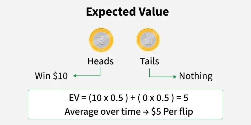
Expected Value Calculation with a Coin Flip — This simple example illustrates the core idea of a weighted average. The expected value isn't necessarily a possible outcome (you can't win $5 in one flip), but it represents the long-term average payout.

Calculating Expected Value for Discrete Variables

For a discrete random variable $X$ that can take values $x_{1}, x_{2}, \dots, x_{n}$ with probabilities $P (X = x_{1}), P (X = x_{2}), \dots, P (X = x_{n})$ , the expected value is the sum of each value multiplied by its probability:

$E [X] = \sum_{i = 1}^{n} x_{i} P (X = x_{i})$

Let's watch a video that walks through this definition and a clear example.

The Expected Value and Variance of Discrete Random Variables

This video from the jbstatistics channel, 'The Expected Value and Variance of Discrete Random Variables', provides an excellent, clear explanation of expected value and how to calculate it for a discrete random variable.

Watch the segments from 00:43 to 02:24 and 04:27 to 06:08. The first part defines expected value, and the second part applies the formula to a concrete example of a biased coin toss.

From Theoretical Expectation to Sample Mean

It's important to distinguish between the theoretical expected value of a random variable's distribution and the sample mean of a dataset.

Expected Value $E [X]$ : A property of the probability distribution itself. It's a constant.
Sample Mean $\overset{x}{ˉ}$ : An estimate of the expected value calculated from a finite sample of data. It's a variable that changes depending on the sample.

Given your background in software engineering, you've likely used functions to calculate the mean of a list of numbers. In Python with NumPy, this is straightforward.

A Gentle Introduction to Expected Value, Variance, and Covariance with NumPy

This article, 'A Gentle Introduction to Expected Value, Variance, and Covariance' by Machine Learning Mastery, provides a clear definition and practical NumPy examples.

Read the section 'Expected Value'. Pay attention to the distinction between the probability-weighted sum (theoretical expectation) and the simple average (sample mean). Also, review the Python code showing how to use numpy.mean().

The numpy.mean() function calculates the sample mean. The Law of Large Numbers (which we will cover in the next lesson) formally states that as your sample size grows, the sample mean will converge to the theoretical expected value.

Calculating Expected Value for Continuous Variables

For a continuous random variable, the concept is the same, but the summation is replaced by an integral over the probability density function (PDF), $f (x)$ :

$E [X] = \int_{- \infty}^{\infty} x f (x) d x$

This integral represents the "center of mass" of the area under the PDF curve.

Deriving the Mean and Variance of a Continuous Probability Distribution

Let's watch another video from jbstatistics, this time demonstrating the calculation for a continuous random variable.

Watch from 00:43 to 03:01. This section shows how to set up and solve the integral to find the expected value for a given PDF. Your experience with calculus from your engineering studies should make this familiar.

2. Variance: The Spread of Outcomes

While expected value tells us about the center of a distribution, it doesn't tell us anything about how spread out the values are. That's the job of variance.

Variance, denoted as $Va r (X)$ or $σ^{2}$ , measures the average squared difference of a random variable from its mean. A small variance means the outcomes are tightly clustered around the expected value, while a large variance means they are widely scattered.

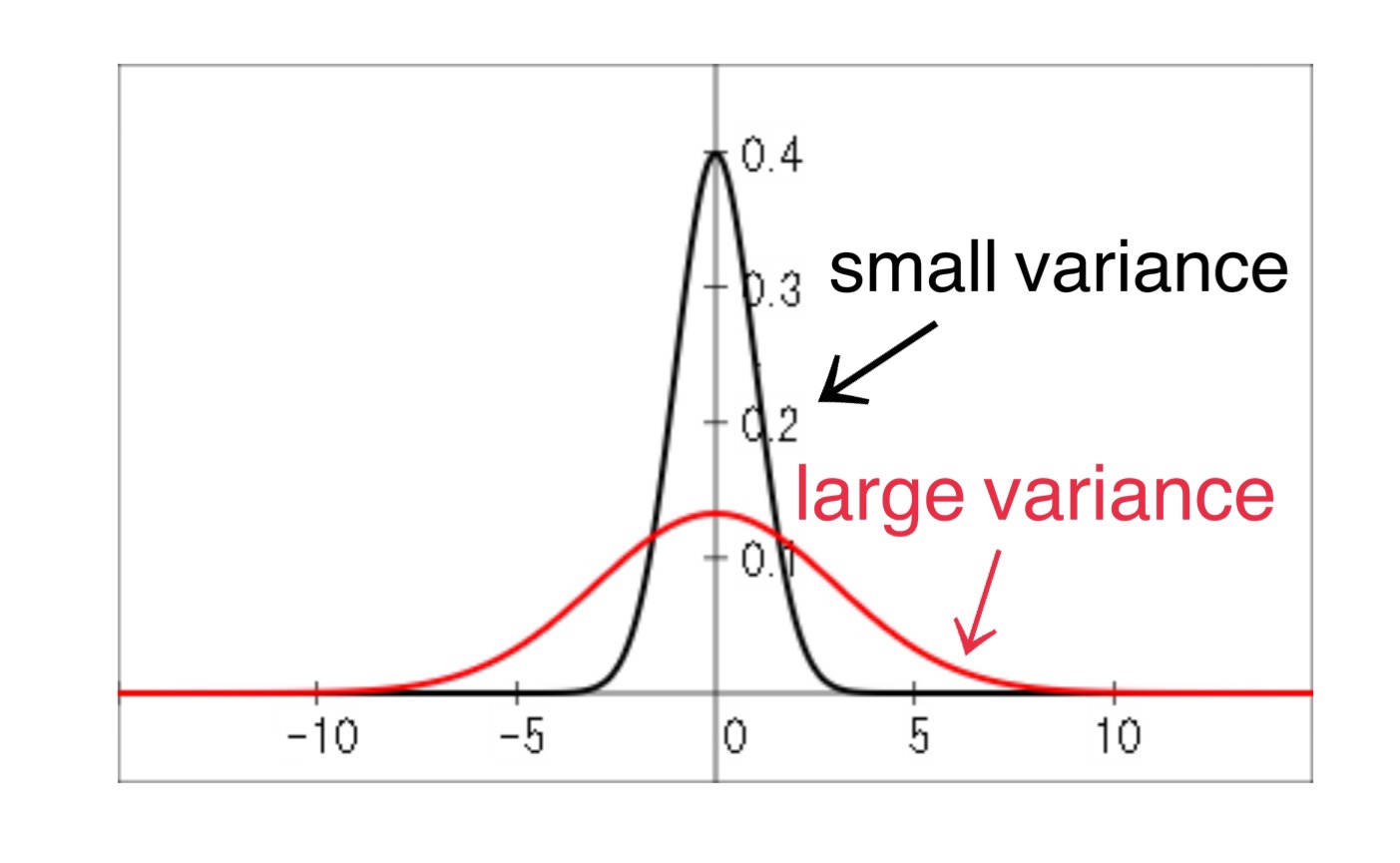
Gaussian Distributions with Small and Large Variance — This image provides a clear visual intuition for variance. Both distributions have the same mean (center), but the red curve has a larger variance, indicating greater uncertainty or spread in the outcomes.

Calculating Variance

The definition of variance is the expectation of the squared deviation from the mean $μ = E [X]$ :

$Va r (X) = E [(X - μ)^{2}]$

For discrete variables, this becomes:
$Va r (X) = \sum_{i = 1}^{n} (x_{i} - μ)^{2} P (X = x_{i})$

For continuous variables, this becomes:
$Va r (X) = \int_{- \infty}^{\infty} (x - μ)^{2} f (x) d x$

While this formula is definitionally pure, a more computationally convenient formula exists:

$Va r (X) = E [X^{2}] - (E [X])^{2}$

This formula states that the variance is the "mean of the square minus the square of the mean." To use it, you first calculate $E [X^{2}]$ and $E [X]$ , then plug them in.

Let's see how both formulas are used in practice.

The Expected Value and Variance of Discrete Random Variables

We'll return to the jbstatistics videos, which do an excellent job of demonstrating the calculation of variance using both the definitional and computational formulas.

First, watch the explanation for the discrete case from 02:50 to 04:12 and 07:26 to 11:10. This covers the two formulas and then applies both to the coin toss example, showing they yield the same result.

Deriving the Mean and Variance of a Continuous Probability Distribution

Now, let's see the same concept applied to the continuous case.

Watch from 03:01 to 07:17. This section walks through calculating E[X²] via integration and then uses the computational formula Var(X) = E[X²] - (E[X])² to find the variance.

Standard Deviation

The standard deviation, denoted $σ$ , is simply the square root of the variance:
$σ = Va r (X)$
The primary advantage of using standard deviation is that it has the same units as the random variable $X$ , making it more interpretable as a typical amount of deviation from the mean.

As with the mean, NumPy provides a simple way to calculate the variance and standard deviation of a sample of data.

A Gentle Introduction to Expected Value, Variance, and Covariance with NumPy

Let's revisit the Machine Learning Mastery article to see the practical implementation.

Read the section 'Variance'. Note the ddof (Delta Degrees of Freedom) parameter in numpy.var(). Setting ddof=1 calculates the sample variance, which is an unbiased estimator for the population variance. This is a subtle but important point in statistics.

Test your understanding!

You are playing a game with a single six-sided die. However, the die is loaded. The probability of rolling each number is as follows:

Outcome (X)	1	2	3	4	5	6
P(X=x)	0.1	0.1	0.1	0.1	0.1	0.5

Calculate the expected value $E [X]$ and the variance $Va r (X)$ of a single roll.

Show answer

1. Calculate the Expected Value $E [X]$ :
We use the formula $E [X] = \sum x \cdot P (X = x)$ .
$E [X] = (1 \cdot 0.1) + (2 \cdot 0.1) + (3 \cdot 0.1) + (4 \cdot 0.1) + (5 \cdot 0.1) + (6 \cdot 0.5)$
$E [X] = 0.1 + 0.2 + 0.3 + 0.4 + 0.5 + 3.0 = 4.5$
The expected value of a roll is 4.5.

2. Calculate the Variance $Va r (X)$ :
We'll use the computational formula $Va r (X) = E [X^{2}] - (E [X])^{2}$ . First, we need to find $E [X^{2}]$ .
$E [X^{2}] = \sum x^{2} \cdot P (X = x)$
$E [X^{2}] = (1^{2} \cdot 0.1) + (2^{2} \cdot 0.1) + (3^{2} \cdot 0.1) + (4^{2} \cdot 0.1) + (5^{2} \cdot 0.1) + (6^{2} \cdot 0.5)$
$E [X^{2}] = (1 \cdot 0.1) + (4 \cdot 0.1) + (9 \cdot 0.1) + (16 \cdot 0.1) + (25 \cdot 0.1) + (36 \cdot 0.5)$
$E [X^{2}] = 0.1 + 0.4 + 0.9 + 1.6 + 2.5 + 18.0 = 23.5$
Now, we plug this into the variance formula:
$Va r (X) = E [X^{2}] - (E [X])^{2} = 23.5 - (4.5)^{2}$
$Va r (X) = 23.5 - 20.25 = 3.25$
The variance of a roll is 3.25. The standard deviation would be $3.25 \approx 1.80$ .

3. Properties of Expectation and Variance

Understanding how expectation and variance behave under transformations is crucial in machine learning. Let $X$ be a random variable and $a, c$ be constants.

ECE 595: Machine Learning I Tutorial 02: Probability Review

This short review from Purdue University provides a concise summary of the key properties of expectation and variance.

Review slides 12 ('Properties of Expectation') and 13 ('Properties of Variance'). Focus on understanding the rules for scaling and shifting a random variable.

Here's a summary of the most important properties:

Properties of Expectation:

Linearity: $E [a X + c] = a E [X] + c$ . This is highly intuitive. If you scale a variable and shift it, its average scales and shifts the same way.
Sum of Variables: $E [X + Y] = E [X] + E [Y]$ . The expectation of a sum is the sum of the expectations. This holds even if $X$ and $Y$ are dependent.

Properties of Variance:

DC Shift: $Va r (X + c) = Va r (X)$ . Adding a constant shifts the entire distribution but does not change its spread. The variance is unchanged.
Scale: $Va r (a X) = a^{2} Va r (X)$ . Scaling a variable by $a$ scales its variance by $a^{2}$ . The square is important; since variance is in squared units, the scaling factor is also squared.
Combined: $Va r (a X + c) = a^{2} Va r (X)$ .

These properties are used extensively in proofs and derivations for ML algorithms, such as analyzing the effects of batch normalization or weight initialization.

Conclusion

In this lesson, we moved from describing distributions to summarizing them numerically. You learned how to compute the two most important summary statistics for any random variable.

Key Takeaways:

Expected Value ( $E [X]$ ) is the probability-weighted average of a random variable's outcomes, representing its center or theoretical mean.
Variance ( $Va r (X)$ ) is the expected squared deviation from the mean, quantifying the spread or dispersion of the outcomes.
The calculation method depends on the variable type: summation for discrete variables and integration for continuous variables.
A computationally efficient formula for variance is $Va r (X) = E [X^{2}] - (E [X])^{2}$ .
Expectation is a linear operator ( $E [a X + c] = a E [X] + c$ ), while variance is not ( $Va r (a X + c) = a^{2} Va r (X)$ ).

Preview of the next lesson:
We have now established a clear difference between the theoretical mean ( $E [X]$ ) of a distribution and the sample mean ( $\overset{x}{ˉ}$ ) calculated from data. But how are they related? How can we be sure that our sample mean is a good estimate of the true, underlying theoretical mean? The next lesson will answer this by exploring two cornerstone theorems of statistics: the Law of Large Numbers and the Central Limit Theorem. These theorems provide the formal justification for why we can use statistics from a sample to make inferences about an entire population or distribution.